The trace of a true strain tensor gives the natural log of the ratio of the intial and final volumes. For an incompressible material, the ratio is 1 and the log of 1 is zero. So the trace of the tensor should equal zero.
\[ 0.758 - 0.546 - 0.212 = 0 \]
So the volume has not changed.
We need the principal values of the strain tensor.
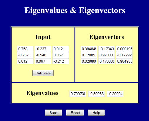
The principal strains are 0.800, -0.600, and -0.200. They add to zero, so \(\epsilon_{\text{Hyd}} = 0.0\).
The max shear is
\[ \begin{eqnarray} \gamma_{\text{Max}} & = & \epsilon_{\text{Max}} - \epsilon_{\text{Min}} \\ \\ & = & 0.800 - (\text{-} 0.600) \\ \\ & = & 1.400 \end{eqnarray} \]
The secondary shear is
\[ \begin{eqnarray} \gamma_{\text{Sec}} & = & \epsilon_{\text{Mid}} - \epsilon_{\text{Hyd}} \\ \\ & = & \text{-} 0.200 - 0.000 \\ \\ & = & \text{-} 0.200 \end{eqnarray} \]
And the ratio of the shears is
\[ { \gamma_{\text{Sec}} \over \;\gamma_{\text{Max}}} \;\; = \;\; {-0.200 \over \;\;\; 1.400} \;\; = \;\; -0.143 \]
So the strain state is close to pure shear, although on the uniaxial tension side of it.
We will need \(\Delta L / L_o\), so get there by taking the exponent of the principal true strain values and subtracting 1.
\[ \begin{eqnarray} \Delta L_1 / L_o & \; = \; & \exp(\;0.800) & - 1 & \; = \; & \;\;1.226 \\ \\ \Delta L_2 / L_o & \; = \; & \exp(-0.600) & - 1 & \; = \; & -0.451 \\ \\ \Delta L_3 / L_o & \; = \; & \exp(-0.200) & - 1 & \; = \; & -0.181 \\ \end{eqnarray} \]
This gives each principal engineering strain value. So the principal engineering strain tensor is
\[ {\bf e}^{\text{Eng}}_\text{Princ} = \left[ \matrix{ 1.226 & \;\;0.0 & \;\;0.0 \\ 0.0 & -0.451 & \;\;0.0 \\ 0.0 & \;\;0.0 & -0.181 } \right] \]
And now the principal strain tensor needs to be rotated back to the proper orientation. This is done by \({\bf e}^\text{Eng} = {\bf Q}^T \cdot {\bf e}^\text{Eng}_\text{Princ} \cdot {\bf Q}\).
The \({\bf Q}\) matrix is in the screen shot above. It is
\[ {\bf Q} = \left[ \matrix{ 0.985 & -0.173 & \;\;\;0.000 \\ 0.171 & \;\;\;0.970 & -0.173 \\ 0.030 & \;\;\;0.170 & \;\;\;0.985 } \right] \]
And the engineering strain tensor is calculated by
\[ \begin{eqnarray} {\bf e}^\text{Eng} & = & \left[ \matrix{ \;\;\;0.985 & \;\;\;0.171 & \;\;\;0.030 \\ -0.173 & \;\;\;0.970 & \;\;\;0.170 \\ \;\;\;0.000 & -0.173 & \;\;\;0.985 } \right] \left[ \matrix{ 1.226 & \;\;0.0 & \;\;0.0 \\ 0.0 & -0.451 & \;\;0.0 \\ 0.0 & \;\;0.0 & -0.181 } \right] \left[ \matrix{ 0.985 & -0.173 & \;\;\;0.000 \\ 0.171 & \;\;\;0.970 & -0.173 \\ 0.030 & \;\;\;0.170 & \;\;\;0.985 } \right] \\ \\ \\ & = & \left[ \matrix{ \;\;\;1.176 & -0.285 & \;\;\;0.008 \\ -0.285 & -0.393 & \;\;\;0.045 \\ \;\;\;0.008 & \;\;\;0.045 & -0.189 } \right] \end{eqnarray} \]
So
\[ \boldsymbol{\epsilon}_{\text{True}} = \left[ \matrix{ \;\;\; 0.758 & -0.237 & \;\;\;0.012 \\ -0.237 & -0.546 & \;\;\;0.067 \\ \;\;\; 0.012 & \;\;\; 0.067 & -0.212 \\ } \right] \qquad \text{corresponds to} \qquad {\bf e}^\text{Eng} = \left[ \matrix{ \;\;\;1.176 & -0.285 & \;\;\;0.008 \\ -0.285 & -0.393 & \;\;\;0.045 \\ \;\;\;0.008 & \;\;\;0.045 & -0.189 } \right] \]
We will need \(\Delta L / L_o\), so get there by taking the exponent of the principal true strain values and subtracting 1.
\[ \begin{eqnarray} \Delta L_1 / L_o & \; = \; & \exp(\;0.800) & - 1 & \; = \; & \;\;1.226 \\ \\ \Delta L_2 / L_o & \; = \; & \exp(-0.600) & - 1 & \; = \; & -0.451 \\ \\ \Delta L_3 / L_o & \; = \; & \exp(-0.200) & - 1 & \; = \; & -0.181 \\ \end{eqnarray} \]
Each principal Green strain value is \({\Delta L \over L_o} + {1 \over 2} \left( {\Delta L \over L_o} \right)^2\).
\[ \begin{eqnarray} E_1 & = & \;\;1.226 + {1 \over 2} ( 1.226 )^2 & = & \;\;1.977 \\ \\ E_2 & = & -0.451 + {1 \over 2} ( -0.451 )^2 & = & -0.349 \\ \\ E_3 & = & -0.181 + {1 \over 2} ( -0.181 )^2 & = & -0.165 \\ \end{eqnarray} \]
So the principal Green strain tensor is
\[ {\bf E}_{\text{Princ}} = \left[ \matrix{ 1.977 & \;\;0.0 & \;\;0.0 \\ 0.0 & -0.349 & \;\;0.0 \\ 0.0 & \;\;0.0 & -0.165 } \right] \]
And now the principal strain tensor needs to be rotated back to the proper orientation. This is done by \({\bf E} = {\bf Q}^T \cdot {\bf E}_{\text{Princ}} \cdot {\bf Q}\).
The \({\bf Q}\) matrix is in the screen shot above. It is
\[ {\bf Q} = \left[ \matrix{ 0.985 & -0.173 & \;\;\;0.000 \\ 0.171 & \;\;\;0.970 & -0.173 \\ 0.030 & \;\;\;0.170 & \;\;\;0.985 } \right] \]
And the Green strain tensor is calculated by
\[ \begin{eqnarray} {\bf E} & = & \left[ \matrix{ \;\;\;0.985 & \;\;\;0.171 & \;\;\;0.030 \\ -0.173 & \;\;\;0.970 & \;\;\;0.170 \\ \;\;\;0.000 & -0.173 & \;\;\;0.985 } \right] \left[ \matrix{ 1.977 & \;\;0.0 & \;\;0.0 \\ 0.0 & -0.349 & \;\;0.0 \\ 0.0 & \;\;0.0 & -0.165 } \right] \left[ \matrix{ 0.985 & -0.173 & \;\;\;0.000 \\ 0.171 & \;\;\;0.970 & -0.173 \\ 0.030 & \;\;\;0.170 & \;\;\;0.985 } \right] \\ \\ \\ & = & \left[ \matrix{ \;\;\;1.907 & -0.397 & \;\;\;0.005 \\ -0.397 & -0.273 & \;\;\;0.031 \\ \;\;\;0.005 & \;\;\;0.031 & -0.171 } \right] \end{eqnarray} \]
So
\[ \boldsymbol{\epsilon}_{\text{True}} = \left[ \matrix{ \;\;\; 0.758 & -0.237 & \;\;\;0.012 \\ -0.237 & -0.546 & \;\;\;0.067 \\ \;\;\; 0.012 & \;\;\; 0.067 & -0.212 \\ } \right] \qquad \text{corresponds to} \qquad {\bf E} = \left[ \matrix{ \;\;\;1.907 & -0.397 & \;\;\;0.005 \\ -0.397 & -0.273 & \;\;\;0.031 \\ \;\;\;0.005 & \;\;\;0.031 & -0.171 } \right] \]
And recall
\[ \boldsymbol{\epsilon}_{\text{True}} = \left[ \matrix{ \;\;\; 0.758 & -0.237 & \;\;\;0.012 \\ -0.237 & -0.546 & \;\;\;0.067 \\ \;\;\; 0.012 & \;\;\; 0.067 & -0.212 \\ } \right] \qquad \text{corresponds to} \qquad {\bf e}^\text{Eng} = \left[ \matrix{ \;\;\;1.176 & -0.285 & \;\;\;0.008 \\ -0.285 & -0.393 & \;\;\;0.045 \\ \;\;\;0.008 & \;\;\;0.045 & -0.189 } \right] \]