Introduction
Metal plasticity research is generally considered to have begun in 1864 with Tresca's publication of his maximum shear stress criterion for yielding. Since then, it has expanded to include effects of anisotropy, rate dependence, and microscopic effects due to grains, dislocations, and atomic slip planes.This page will first cover the fundamental mechanisms of plastic deformations, which occur at the atomic scale. It will then move to macroscale models of plasticity. Macroscale approaches treat metals as isotropic continuums down to the smallest scales possible. It starts with 1-D applications, which will seem ridiculously simple, but will allow fundamental principles to be introduced. It then moves to 3-D applications.
Fundamental Mechanisms
The key fundamental mechanism of metal plasticity is movement of atoms along atomic slip planes. For example, in the 2-D figure below, the circles represent atoms packed together in a metal. The metal is subjected to a macroscopic shear stress as shown. As is the usual case, the external loading does not line up with the slip planes. This makes the deformation mechanisms at the microscopic scale quite complicated.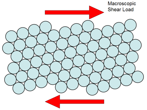
There are three major slip planes in this 2-D example. (There are many more in the real 3-D world.) They are identified in the sketch below. Each slip plane has a unit normal vector, \({\bf n}_i\), and a slip direction vector, \({\bf s}_i\).
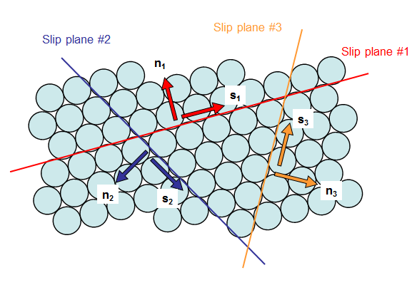
Slip does not occur on the slip plane unless the resolved shear stress on the slip plane exceeds the critical resolved shear stress of the material. The resolved shear stress is calculated by
\[ \tau_\text{resolved} = \sigma_{ij} s_i n_j \]
It should be clear in this example that as the external shear load is increased, the resolved shear stress on slip plane #1 will grow the most rapidly and trigger slip on this plane first, long before (if at all) the other slip systems become active.
The net result is that all the slip planes parallel to #1 begin to shear, producing
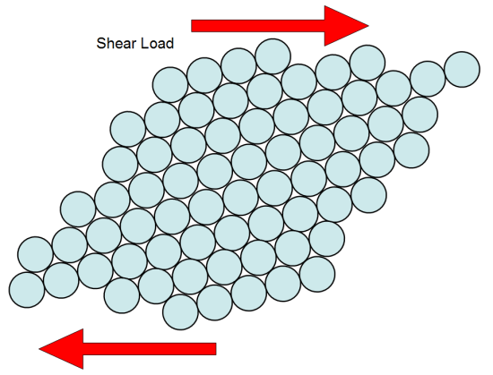
This is usually accompanied by rotation of the slip planes too. It should be clear that the process does not change the volume of the material. That is why plasticity is incompressible (as established beyond any doubt in tests performed by Bridgeman in 1947 and 1952). Also, as the atoms slide, dislocations (glitches in the atomic stack-ups) grow in number and raise the critical resolved shear stress required to maintain further plastic deformation. This accounts for the gradual increase in stress with continued plastic deformation.
All of this is just for a single grain. This makes it very anisotropic because any applied shear that aligns with a slip plane will produce a lower yield stress than an applied shear that does not align. But unless you are a turbine blade, then the metal is actually made up of millions or billions of randomly oriented grains. This is represented schematically as shown below.
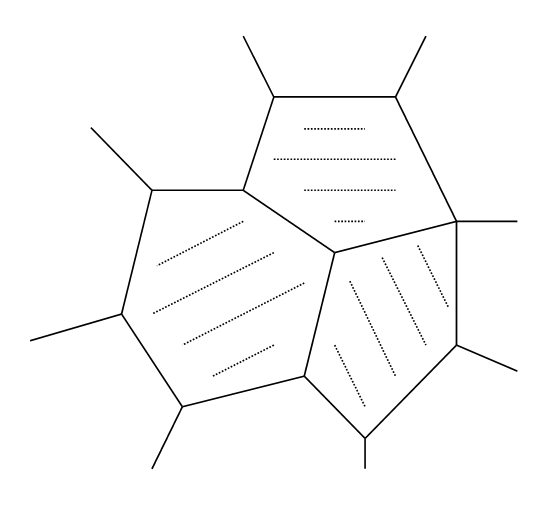
This results in initially isotropic behavior at the macroscale. The measured yield stress is the same regardless of the loading direction. But as a metal is plastically deformed, the slip planes rotate and align with each other, producing anisotropic material properties. (The grain shapes themselves have no impact on the plastic behavior. Only the slip planes orientations matter.)
These mechanisms are relatively easy to understand, but it turns out that they are fantastically hard to actually model and calculate in 3-D. For starters, it is necessary to partition the total deformation, represented by \({\bf F}\), into portions due to plastic deformations, \({\bf F^p}\), followed by elastic deformations, \({\bf F^e}\). This is attributed to Lee (1969) and written as
\[ {\bf F} = {\bf F^e} \cdot {\bf F^p} \]
Note that just like with the polar decompositions, the matrices are read from right to left. So in this case, the plastic deformation is assumed to take place first, followed by the elastic deformations.
1-D Metal Plasticity
The complexity of microscale descriptions of metal plasticity, polycrystal plasticity, is why for 99.99% of applications, macroscale plasticity theories are used. These are very empirical. They are based solely on observed behaviors at the macroscale.This process begins with simple uniaxial stress-strain curves as follows.
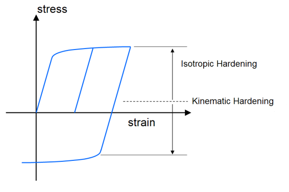
The graph shows so-called isotropic and kinematic hardening that takes place in metals. The kinematic aspect is the anisotropic part that is responsible for the center of the yield surface drifting away from zero. This is sometimes called the Bauschinger effect after the researcher that first identified it in 1881. The isotropic aspect is symmetric regardless of the direction of loading.
This is relatively easy to work with in 1-D. The elastic strain, \(\epsilon^{el}\), is
\[ \epsilon^{el} = {\sigma \over E} \]
\[ \epsilon^{pl} = K \sigma^m \]
The total strain is the sum of the two
\[ \epsilon = {\sigma \over E} + K \sigma^m \]
Just keep in mind that the plastic part is completely empirical. It is only a curve-fit, and only good for 1-D applications where the strains are relatively small because the single exponent, m, cannot fit data over large strain ranges.
3-D Metal Plasticity
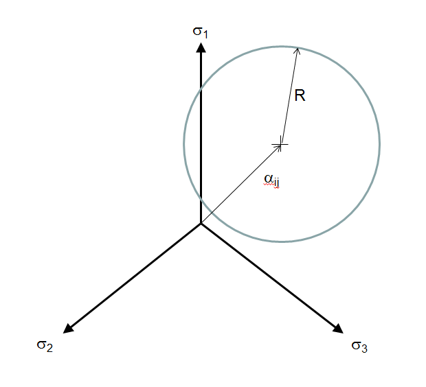
The situation is significantly more complex in 3-D. In this case, yielding is dictated by the von Mises stress. Recall that this is a circle, as in the following sketch.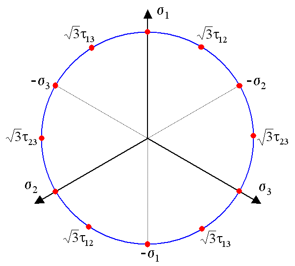
Note that the above sketch is for the purely isotropic case. Kinematic hardening is represented by the circle moving away from the origin. Since this occurs in stress space, the circle's center is described by a traceless stress tensor, \(\alpha_{ij}\), called the backstress tensor, or kinematic hardening variable.