Introduction
It is the well known governing differential equation of fluid flow, and usually considered intimidating due to its size and complexity. The objective here is not to solve it, but to show that it is in fact based on only a few simple key concepts.
We will see that the Navier-Stokes equation is only a small step forward in continuum mechanics. It is a combination of the continuity equation, the equilibrium equation, the material derivative, and the rate of deformation tensor, all of which we have already covered.
Navier-Stokes Equation
The development below gets relatively involved algebraically. Nevertheless, the key concepts are straight-forward. They are summarized here.- The starting point of the Navier-Stokes equations is the equilibrium equation.
- The first key step is to partition the stress in the equations into hydrostatic (pressure) and deviatoric constituents.
- The second step is to relate the deviatoric stress to viscosity in the fluid.
- The final step is to impose any special cases of interest, usually incompressibility.
Start with the equilibrium equation.
\[ \nabla \cdot \boldsymbol{\sigma} + \rho \, {\bf f} = \rho \, {\bf a} \qquad \qquad \sigma_{ij,j} + \rho f_i = \rho \, a_i \]
And insert the material derivative for the acceleration term
\[ \nabla \cdot \boldsymbol{\sigma} + \rho \, {\bf f} = \rho \, \left( {\partial {\bf v} \over \partial t} + {\bf v} \cdot \nabla {\bf v} \right) \qquad \qquad \sigma_{ij,j} + \rho f_i = \rho \, ( v_{i,t} + v_k v_{i,k} ) \]
Partition the stress into the sum of its hydrostatic and deviatoric parts, but express the hydrostatic part as pressure.
\[ \boldsymbol{\sigma} = -P \, {\bf I} + \boldsymbol{\sigma}' \]
Insert this back into the equilibrium equation.
\[ -\nabla P + \nabla \cdot \boldsymbol{\sigma}' + \rho \, {\bf f} = \rho \, \left( {\partial {\bf v} \over \partial t} + {\bf v} \cdot \nabla {\bf v} \right) \]
Up until this point, the equilibrium equation is still completely general. It still applies to all materials, solid or liquid. But the next step commits us to the Navier-Stokes equation because we introduce a constitutive model of viscous fluid flow into the equation. That constitutive model relates the deviatoric stress to the shear strain rate, i.e., the deviatoric rate of deformation tensor.
\[ \boldsymbol{\sigma}' = 2 \mu {\bf D}' \]
where \(\mu\) is the fluid's viscosity. (Note the similarity to \(\boldsymbol{\sigma}' = 2 G \boldsymbol{\epsilon}'\) in Hooke's Law.) It is in fact the general 3-D version of the familiar \(\tau = \mu {\partial v_x \over \partial y}\) viscosity relationship. Inserting and rearranging, and assuming \(\mu\) is a constant, gives one of the most general forms of the equation.
\[ \rho \, \left( {\partial {\bf v} \over \partial t} + {\bf v} \cdot \nabla {\bf v} \right) = -\nabla P + 2 \mu \nabla \cdot {\bf D}' + \rho \, {\bf f} \]
And now replace \({\bf D}'\) with \({\bf D} - {1 \over 3} \text {tr}({\bf D}) {\bf I}\). This gives
\[ \rho \, \left( {\partial {\bf v} \over \partial t} + {\bf v} \cdot \nabla {\bf v} \right) = -\nabla P + 2 \mu \nabla \cdot {\bf D} - {2 \over 3} \mu \nabla (\text{tr}({\bf D})) + \rho \, {\bf f} \]
and substitute \({\bf D} = (\nabla {\bf v} + (\nabla {\bf v})^T)/2\).
\[ \rho \, \left( {\partial {\bf v} \over \partial t} + {\bf v} \cdot \nabla {\bf v} \right) = -\nabla P + \mu \nabla^2 {\bf v} + {1 \over 3} \mu \nabla (\nabla \cdot {\bf v}) + \rho \, {\bf f} \]
The continuity equation dictates that \(\nabla \cdot {\bf v} = 0\) for an incompressible material, so the entire \({1 \over 3} \mu \nabla (\nabla \cdot {\bf v})\) term drops out of the Navier-Stokes equation. This leaves
\[ \rho \, \left( {\partial {\bf v} \over \partial t} + {\bf v} \cdot \nabla {\bf v} \right) = -\nabla P + \mu \nabla^2 {\bf v} + \rho \, {\bf f} \]
This is the familiar Navier-Stokes equation. When expanded out, it gives
\[ \rho \, \left( {\partial v_1 \over \partial t} + v_1 {\partial v_1 \over \partial x_1} + v_2 {\partial v_1 \over \partial x_2} + v_3 {\partial v_1 \over \partial x_3} \right) = -{\partial P \over \partial x_1} + \mu \left( {\partial^2 v_1 \over \partial x_1^2} + {\partial^2 v_1 \over \partial x_2^2} + {\partial^2 v_1 \over \partial x_3^2} \right) + \rho \, f_1 \] \[ \rho \, \left( {\partial v_2 \over \partial t} + v_1 {\partial v_2 \over \partial x_1} + v_2 {\partial v_2 \over \partial x_2} + v_3 {\partial v_2 \over \partial x_3} \right) = -{\partial P \over \partial x_2} + \mu \left( {\partial^2 v_2 \over \partial x_1^2} + {\partial^2 v_2 \over \partial x_2^2} + {\partial^2 v_2 \over \partial x_3^2} \right) + \rho \, f_2 \] \[ \rho \, \left( {\partial v_3 \over \partial t} + v_1 {\partial v_3 \over \partial x_1} + v_2 {\partial v_3 \over \partial x_2} + v_3 {\partial v_3 \over \partial x_3} \right) = -{\partial P \over \partial x_3} + \mu \left( {\partial^2 v_3 \over \partial x_1^2} + {\partial^2 v_3 \over \partial x_2^2} + {\partial^2 v_3 \over \partial x_3^2} \right) + \rho \, f_3 \]
Of course, these equations are too intractable to be of any use for providing physical insight or analytical solutions. But that's not the point here. The main point of this exercise was to demonstrate that their complete development is within relatively easy reach using the basic relationships of continuum mechanics that we have already covered.
Dimensionless Numbers
It is the simple case of particle position with an initial velocity and undergoing constant acceleration. The position is given by the familiar equation.
\[ s = v_o t + {1 \over 2} a \, t^2 \]
This is a convenient example problem because it is simple and it is clear that the position is the sum of a velocity term and an acceleration term, either of which may be dominant in a given problem. The first step is to introduce dimensionless parameters for all the variables. For example, \(s^* = s / L\), where \(s^*\) is the dimensionless parameter, \(s\) is the usual position variable, and \(L\) is a characteristic length.
\[ s^* = s / L \qquad \quad v^* = v_o / V \qquad \quad a^* = a / A \qquad \quad t^* = t / T \]
Rearrangement gives
\[ s = s^* L \qquad \quad v_o = v^* V \qquad \quad a = a^* A \qquad \quad t = t^* T \]
and substitution into the original equation gives
\[ s^* L = v^* V \, t^* T + {1 \over 2} a^* A \, (t^* T)^2 \]
Regroup
\[ \left( {L \over V \, T} \right) s^* = v^* t^* + {1 \over 2} a^* {t^*}^2 \left( {A \, T \over V} \right) \]
This gives two dimensionless parameters, \({L \over V \, T}\) and \({A \, T \over V}\). As is often the case, the dimensionless numbers appear as ratios of parameters. In this case, \({A \, T \over V}\) is the ratio of acceleration effects to the initial velocity.
The next step is to conduct experimental tests to determine the system's behavior. In this hypothetical case, different values would be chosen for velocity, acceleration, and time in the experiment, and then the displacement would be measured. But we will simply calculate the actual displacement using the original equation. Choosing random input values yields the following results, including the dimensionless numbers.
| vo | a | t | s | AT/V | L/VT |
|---|---|---|---|---|---|
| 0.1 | 0 | 3 | 0.3 | 0.00 | 1.00 |
| -3 | 25 | 1 | 9.5 | -8.33 | -3.17 |
| 2 | 9.8 | 2 | 23.6 | 9.80 | 5.90 |
| -10 | 5 | 2 | -10 | -1.00 | 0.50 |
| 7 | 60 | 1 | 37 | 8.57 | 5.29 |
| 20 | 10 | 9 | 585 | 4.50 | 3.25 |
| -1 | -2 | 3 | -12 | 6.00 | 4.00 |
| 3 | -4 | 1 | 1 | -1.33 | 0.33 |
| -5 | -6 | 2 | -22 | 2.40 | 2.20 |
| 4 | -7 | 2 | -6 | -3.50 | -0.75 |
| -8 | -20 | 1 | -18 | 2.50 | 2.25 |
| 20 | -15 | 9 | -427.5 | -6.75 | -2.38 |
Now plot the two dimensionless numbers against each other. The result is pretty amazing.
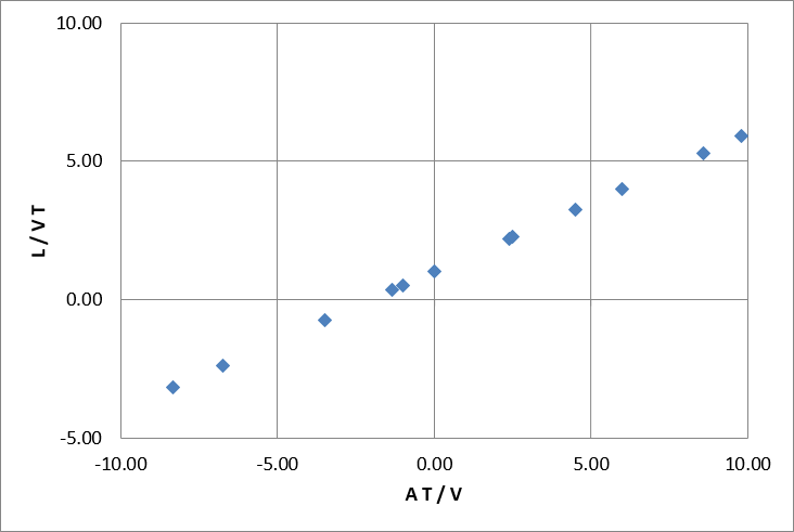
The test points form a well defined master-curve (in this case, a simple line) when plotted as dimensionless numbers. It makes it possible to compute \((A \, T / V)\) for any problem and go to this chart to obtain the corresponding \((L / V \, T)\), and from this, finally determine \(L\).
Reynolds Number
The same process of defining dimensionless parameters and inserting them into the governing equations yield the dimensionless numbers that govern fluid flow. Start with\[ \rho \, \left( {\partial {\bf v} \over \partial t} + {\bf v} \cdot \nabla {\bf v} \right) = -\nabla P + \mu \nabla^2 {\bf v} + \rho \, {\bf f} \]
Assume steady state, negligible body forces, and write the equation somewhat less rigorously as
\[ \rho \, v \, {\partial v \over \partial x} = - {\partial P \over \partial x} + \mu {\partial^2 v \over \partial x^2} \]
Define the following dimensionless parameters.
\[ \rho^* = \rho / R \qquad \quad v^* = v / V \qquad \quad x^* = x / L \qquad \quad p^* = p / \Delta P \qquad \quad \mu^* = \mu / M \]
Rearrangement gives
\[ \rho = \rho^* R \qquad \quad v = v^* V \qquad \quad x = x^* L \qquad \quad p = p^* \Delta P \qquad \quad \mu = \mu^* M \]
and substitution into the equation gives
\[ \rho^* R \, v^* V \, {\partial (v^* V) \over \partial (x^* L)} = - {\partial (P^* \Delta P) \over \partial (x^* L)} + \mu^* M {\partial^2 (v^* V) \over \partial (x^* L)^2} \]
Regrouping gives
\[ \left({ R V^2 \over L}\right) \rho^* v^* {\partial v^* \over \partial x^* } = - \left( {\Delta P \over L} \right) {\partial P^* \over \partial x^* } + \left( {M V \over L^2} \right) \mu^* {\partial^2 v^* \over \partial {x^*}^2} \]
Divide through by \(R V^2 / L\) to get
\[ \rho^* v^* {\partial v^* \over \partial x^* } = - \left( {\Delta P \over R V^2} \right) {\partial P^* \over \partial x^* } + \left( {M \over R V L} \right) \mu^* {\partial^2 v^* \over \partial {x^*}^2} \]
(Recall that \(R\) is density, \(\rho\), and \(M\) is viscosity, \(\mu\)). This means that the two dimensionless numbers are
\[ N = {\Delta P \over \rho V^2} \qquad \qquad Re = {\rho V L \over \mu} \]
The Reynolds number is the ratio of inertial forces to viscous forces. Inertial forces are related to \(\rho V^2\). Viscous forces are related to \(\mu V / L\). The ratio is
\[ { \rho V^2 \over \mu \left( { V \over L} \right) } = {\rho V L \over \mu} = Re \]
The Navier-Stokes equation can be written as
\[ \rho^* v^* {\partial v^* \over \partial x^* } = - N {\partial P^* \over \partial x^* } + {1 \over Re} \mu^* {\partial^2 v^* \over \partial {x^*}^2} \]
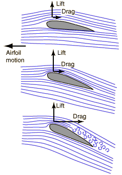
High Reynolds numbers reflect the fact that inertial forces are much higher than viscous forces. This usually occurs when the velocities are high. In this case, the viscosity terms in the above equation become negligible. This is typical of hydroplaning, which takes place when the inertia of the water just in front of the contact patch resists the tread blocks' efforts to push it out of the way.
The opposite case, low Reynolds numbers, reflect the case where viscosity forces dominate. This occurs during viscoplaning when the film of water between the tread blocks and road surface is trapped between such a small gap that any flow results in high velocity gradients that produce large viscosity forces.
Bernoulli Equation
\[ {\bf v} \cdot \nabla {\bf v} = {1 \over 2} \nabla {\bf v}^2 - {\bf v} \times (\nabla \times {\bf v}) \]
Substituting it into the Navier-Stokes equation gives
\[ \rho \, \left( {\partial {\bf v} \over \partial t} + {1 \over 2} \nabla {\bf v}^2 - {\bf v} \times (\nabla \times {\bf v}) \right) = -\nabla P + \mu \nabla^2 {\bf v} + \rho \, {\bf f} \]
Now the simplifications. First, assume that the fluid flow is steady-state, so \({\partial {\bf v} \over \partial t} = 0\). Second, neglect the viscous term. And finally, assume the fluid is irrotational, \(\nabla \times {\bf v} = 0\). This leaves
\[ {1 \over 2} \rho \nabla {\bf v}^2 = -\nabla P + \rho \, {\bf f} \]
And the body force term must be tackled. For this case, it is gravity acting in the \(-z\) direction. It is usually written as
\[ \rho \, {\bf f} = - \rho \, g \, {\bf k} \]
But for development of the Bernoulli equation, we will instead write it as
\[ \rho \, {\bf f} = - \nabla (\rho g z) \]
Substituting this gives
\[ {1 \over 2} \rho \nabla {\bf v}^2 = -\nabla P - \nabla (\rho g z) \]
And rearrange to get
\[ \nabla \left( {1 \over 2} \rho {\bf v}^2 + P + \rho g z \right) = 0 \]
Which means that the term inside the parentheses must be a constant.
\[ {1 \over 2} \rho {\bf v}^2 + P + \rho g z = const \]
This is the classical Bernoulli equation, first proposed by Daniel Bernoulli in 1738. It is basically the conservation of kinetic and potential energy from high school physics classes, plus the pressure term, essentially an internal energy component.
The terms in the equation have many names, and combinations of the terms have still more names. \(P\) is the static pressure, even if the fluid is moving. \({1 \over 2} \rho {\bf v}^2\), the kinetic term, is dynamic pressure. It is the pressure one feels when the wind blows on you. Technically, it is the pressure you feel due to the wind being brought from velocity, \(V\), down to zero, since it can't pass through you. The static and dynamic pressure together give the total or stagnation pressure.
Dividing the equation through by \(\rho g\) transforms it from an equation in units of pressure to one in terms of height, \(z\).
\[ {\; {\bf v}^2 \over 2 g} + {P \over \rho g} + z = H \]
In this form, the constant is called the total head of the flow, and represented by the letter, \(H\). It allows the energy of the flow field to be expressed in units of height.
Recall that viscous effects were neglected in the derivation of Bernoulli's equation. But of course, they are present in real world applications. The net effect of fluid viscosity is to decrease the constant in the equation, effectively reducing the energy of the flow field. This is usually called head loss. For flow through a pipe, the viscosity produces a pressure drop, or head loss along the length of the pipe. The head loss can be calculated with the aid of a Moody Chart. The second step, yes second, is to compute the head loss with this equation.
\[ \Delta H = f_D \left( {L \over D} \right) {V^2 \over 2 g} \]
Where \(f_D\) is the Darcy friction factor that is first determined from the Moody Diagram

It satisfies the following Colebrook equation (that requires iterative solution) for transitional and fully turbulent flows.
\[ {1 \over \sqrt{f \,}} = -2 \, \log_\text{10} \left( {\epsilon \over 3.7 \, D_h} + {2.51 \over Re \sqrt{f \,}} \right) \]
At room temperature, water's viscosity is 9*10-4 Pa-sec and air's viscosity is 1.9*10-5 Pa-sec.
Many fluid viscosity values are listed on this page: http://en.wikipedia.org/wiki/Viscosity.
City Water
Our local government recently ran "city water" to our neighborhood. We had a choice between 3/4" (19 mm) or 1" (25 mm) diameter pipe to run from the road to the house. The water pressure through the main line at the road is 60 psi (414,000 Pa), I think. The house is about 100 ft (30 m) from the road. What is the flow rates we can expect from each pipe?The "head" for 60 psi (= 414,000 Pa) is \(P / \rho g\).
\[ {P \over \rho g} = { 414,000\text{ Pa} \over (1,000 \text{kg/m}^3) \; (9.8 \text{m/s}^2) } = 42.2\text{m} \]
For plastic pipes, the table in the lower left corner of the Moody Diagram says that surface roughness is 0.0025 mm. The ratio of roughness to pipe diameter, for the 1" pipe, is 0.0025 mm/25 mm = 1E-4. The friction factor is 0.013. The velocity corresponding to 42.2 m head is
\[ 42.2\text{m} = {0.013 \over 2} \left( { 30\text{m} \over 0.025\text{m} } \right) \left( {V^2 \over 9.8\text{m/s}^2 } \right) \]
The velocity is 7.3 m/s. Now calculate the Reynolds number.
\[ Re = {\rho V D \over \mu} = { (1000\text{kg/m}^3) (7.3\text{m/s}) (0.025\text{m}) \over 9(10)^{\text{-}4}\text{Pa s} } = 200,000 \]
Double-check this value on the Moody diagram. It turns out that the friction coefficient should be a little higher, about 0.015, but that's close enough for now.
So now calculate the mass flow rate.
\[ \dot m = \rho V A = (1000 \text{kg/m}^3) (7.3\text{m/s}) (5(10)^{\text{-}4}\text{m}^2) = 3.6\text{kg/s} \]
Now redo the calculations for the 3/4" pipe. For plastic pipes, the table in the lower left corner of the Moody Diagram says that surface roughness is 0.0025 mm. The ratio of roughness to pipe diameter, for the 1" pipe, is 0.0025 mm/19 mm = 1.3E-4. The friction factor is 0.015. The velocity corresponding to 42.2 m head is
\[ 42.2\text{m} = {0.015 \over 2} \left( { 30\text{m} \over 0.019\text{m} } \right) \left( {V^2 \over 9.8\text{m/s}^2 } \right) \]
The velocity is 5.9 m/s. The fact that this is smaller than the 7.3 m/s speed of the flow in the 1" pipe reflects the effects of viscosity introducing greater drag in the smaller pipe than the bigger one.
Now calculate the Reynolds number.
\[ Re = {\rho V D \over \mu} = { (1000\text{kg/m}^3) (5.9\text{m/s}) (0.019\text{m}) \over 9(10)^{\text{-}4}\text{Pa s} } = 125,000 \]
Double-check this value on the Moody diagram. It turns out that the friction coefficient should be a little higher, about 0.017, but that's close enough for now as well.
Now calculate the mass flow rate.
\[ \dot m = \rho V A = (1000 \text{kg/m}^3) (5.9\text{m/s}) (2.9(10)^{\text{-}4}\text{m}^2) = 1.7\text{kg/s} \]
This is 47% of the mass flow rate of the 1" pipe, even though the 3/4" pipe's area is 56% of the 1" pipe's area. I'm glad we chose the 1" pipe.