Search Continuum Mechanics Website

Principal Stresses & Strains

 home > introductory mechanics > principal stresses & strains

Introduction

This page covers principal stresses and strains. Although we have not yet discussed the many different definitions of stress and strain, it is in fact true that everything discussed here applies regardless of the type of stress or strain tensor. For example, if you calculate the principal values of a Cauchy stress tensor, then what you get are principal Caucy stresses. The principal values of a Green strain tensor will be principal Green strains.

Everything below follows from two facts: First, the input stress and strain tensors are symmetric. Second, the coordinate transformations discussed here are applicable to stress and strain tensors (they indeed are).

We will talk about stress first, then strain.

---

2-D Principal Stresses

In 2-D, the transformation equations are

\[ \begin{eqnarray} \sigma'\!_{xx} & = & \sigma_{xx} \cos^2 \theta + \sigma_{yy} \, \sin^2 \theta + 2 \, \tau_{xy} \, \sin \theta \cos \theta \\ \\ \sigma'\!_{yy} & = & \sigma_{xx} \sin^2 \theta + \sigma_{yy} \, \cos^2 \theta - 2 \, \tau_{xy} \, \sin \theta \cos \theta \\ \\ \tau'\!_{xy} & = & (\sigma_{yy} - \sigma_{xx}) \sin \theta \cos \theta + \tau_{xy} (\cos^2 \theta - \sin^2 \theta) \end{eqnarray} \]
These are the expanded forms of \(\boldsymbol{\sigma}' = {\bf Q} \cdot \boldsymbol{\sigma} \cdot {\bf Q}^T\) in 2-D. They can also be derived from a force balance of the figure shown here. It is interesting that stress is characterized as a tensor because it follows the transformation equation. But this is primarily a mathematical argument, and it would carry little weight if it were not connected to the physics of the force balance. The fact that the coordinate transform equation properly reflects the force balance at different orientations is what makes it relevant.

The principal stresses are the corresponding normal stresses at an angle, \(\theta_P\), at which the shear stress, \(\tau'_{xy}\), is zero.

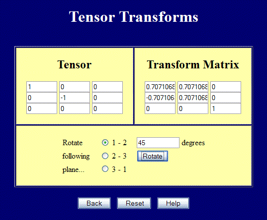
This page performs full 3-D tensor transforms, but can still be used for 2-D problems.. Enter values in the upper left 2x2 positions and rotate in the 1-2 plane to perform transforms in 2-D. The screenshot below shows a case of pure shear rotated 45° to obtain the principal stresses. Note also how the \({\bf Q}\) matrix transforms.



The figure below shows the stresses corresponding to the pure shear case in the tensor transform webpage example. The blue square aligned with the axes clearly undergoes shear. But the red square inscribed in the larger blue square only sees simple tension and compression. These are the principal values of the pure shear case in the global coordinate system.



In 2-D, the principal stress orientation, \(\theta_P\), can be computed by setting \(\tau'\!_{xy} = 0\) in the above shear equation and solving for \(\theta\) to get \(\theta_P\), the principal stress angle.

\[ 0 = (\sigma_{yy} - \sigma_{xx}) \sin \theta_P \cos \theta_P + \tau_{xy} (\cos^2 \theta_P - \sin^2 \theta_P) \]
This gives

\[ \tan (2 \theta_P) \; = \; {2 \tau_{xy} \over \sigma_{xx} - \sigma_{yy} } \]
The transformation matrix, \({\bf Q}\), is

\[ {\bf Q} = \left[ \matrix{ \;\;\; \cos \theta_P & \sin \theta_P \\ -\sin \theta_P & \cos \theta_P } \right] \]
Inserting this value for \(\theta_P\) back into the equations for the normal stresses gives the principal values. They are written as \(\sigma_{max}\) and \(\sigma_{min}\), or alternatively as \(\sigma_1\) and \(\sigma_2\).

\[ \sigma_{max}, \sigma_{min} = {\sigma_{xx} + \sigma_{yy} \over 2} \pm \sqrt{ \left( {\sigma_{xx} - \sigma_{yy} \over 2} \right)^2 + \tau_{xy}^2 } \]
They could also be obtained by using \(\boldsymbol{\sigma}' = {\bf Q} \cdot \boldsymbol{\sigma} \cdot {\bf Q}^T\) with \({\bf Q}\) based on \(\theta_P\).

---

3-D Principal Stresses

Coordinate transforms in 3-D are

\[ \left[ \matrix{\sigma'_{11} & \sigma'_{12} & \sigma'_{13} \\ \sigma'_{12} & \sigma'_{22} & \sigma'_{23} \\ \sigma'_{13} & \sigma'_{23} & \sigma'_{33} } \right] = \left[ \matrix { q_{11} & q_{12} & q_{13} \\ q_{21} & q_{22} & q_{23} \\ q_{31} & q_{32} & q_{33} } \right] \left[ \matrix{\sigma_{11} & \sigma_{12} & \sigma_{13} \\ \sigma_{12} & \sigma_{22} & \sigma_{23} \\ \sigma_{13} & \sigma_{23} & \sigma_{33} } \right] \left[ \matrix { q_{11} & q_{21} & q_{31} \\ q_{12} & q_{22} & q_{32} \\ q_{13} & q_{23} & q_{33} } \right] \]
The second \({\bf Q}\) matrix is once again the transpose of the first.

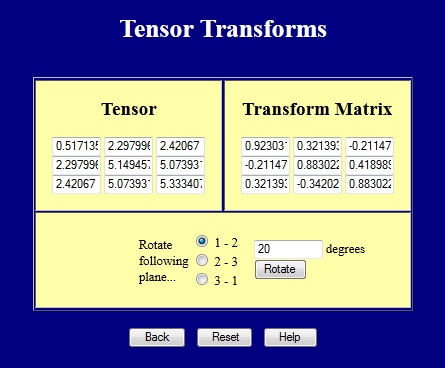
This page performs tensor transforms.



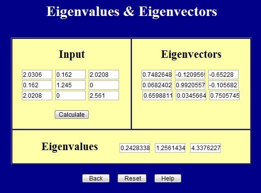
And this page calculates principal values (eigenvalues) and principal directions (eigenvectors).



It's important to remember that the inputs to both pages must be symmetric. In fact, both pages enforce this.

The eigenvalues above can be written in matrix form as

\[ \boldsymbol{\sigma} = \left[ \matrix{ 24 & 0 & 0 \\ 0 & 125 & 0 \\ 0 & 0 & 433 } \right] \]

---

2-D Principal Strains

The mechanics of computing principal strains is identical to that for computing principal stresses. The only potential pitfall to keep in mind is that the equations always operate on one-half of the shear values, \(\gamma / 2\).

In 2-D, the transformation equations are

\[ \begin{eqnarray} \epsilon'\!_{xx} & = & \epsilon_{xx} \cos^2 \theta + \epsilon_{yy} \, \sin^2 \theta + 2 \left( {\gamma_{xy} \over 2} \right) \sin \theta \cos \theta \\ \\ \epsilon'\!_{yy} & = & \epsilon_{xx} \sin^2 \theta + \epsilon_{yy} \, \cos^2 \theta - 2 \left( {\gamma_{xy} \over 2} \right) \sin \theta \cos \theta \\ \\ {\gamma'\!_{xy} \over 2} & = & (\epsilon_{yy} - \epsilon_{xx}) \sin \theta \cos \theta + \left( {\gamma_{xy} \over 2} \right) (\cos^2 \theta - \sin^2 \theta) \end{eqnarray} \]
The equations are written in terms of \(\gamma / 2\) to emphasize that half of all the shear values are used in the transformation equations.

This page performs full 3-D tensor transforms, but can still be used for 2-D problems.. Enter values in the upper left 2x2 positions and rotate in the 1-2 plane to perform transforms in 2-D. The screenshot below shows a case of pure shear rotated 45° to obtain the principal strains. Note also how the \({\bf Q}\) matrix transforms.



The figure below shows the deformed shapes corresponding to the pure shear case in the tensor transform webpage example. The blue square aligned with the axes clearly undergoes shear. But the red square inscribed in the larger blue square only sees simple tension and compression. These are the principal values of the pure shear deformation in the global coordinate system.



In 2-D, the principal strain orientation, \(\theta_P\), can be computed by setting \(\gamma'\!_{xy} = 0\) in the above shear equation and solving for \(\theta\) to get \(\theta_P\), the principal strain angle.

\[ 0 = (\epsilon_{yy} - \epsilon_{xx}) \sin \theta_P \cos \theta_P + \left( {\gamma_{xy} \over 2} \right) (\cos^2 \theta_P - \sin^2 \theta_P) \]
This gives

\[ \tan (2 \theta_P) \; = \; {\gamma_{xy} \over \epsilon_{xx} - \epsilon_{yy} } \; = \; {2 \epsilon_{xy} \over \epsilon_{xx} - \epsilon_{yy} } \]
The transformation matrix, \({\bf Q}\), is

\[ {\bf Q} = \left[ \matrix{ \;\;\; \cos \theta_P & \sin \theta_P \\ -\sin \theta_P & \cos \theta_P } \right] \]
Inserting this value for \(\theta_P\) back into the equations for the normal strains gives the principal values. They are written as \(\epsilon_{max}\) and \(\epsilon_{min}\), or alternatively as \(\epsilon_1\) and \(\epsilon_2\).

\[ \epsilon_{max}, \epsilon_{min} = {\epsilon_{xx} + \epsilon_{yy} \over 2} \pm \sqrt{ \left( {\epsilon_{xx} - \epsilon_{yy} \over 2} \right)^2 + \left( \gamma_{xy} \over 2 \right)^2 } \]
They could also be obtained by using \({\bf E}' = {\bf Q} \cdot {\bf E} \cdot {\bf Q}^T\) with \({\bf Q}\) based on \(\theta_P\).

---

3-D Principal Strains

Coordinate transforms in 3-D are

\[ \left[ \matrix{E'_{11} & E'_{12} & E'_{13} \\ E'_{12} & E'_{22} & E'_{23} \\ E'_{13} & E'_{23} & E'_{33} } \right] = \left[ \matrix { q_{11} & q_{12} & q_{13} \\ q_{21} & q_{22} & q_{23} \\ q_{31} & q_{32} & q_{33} } \right] \left[ \matrix{E_{11} & E_{12} & E_{13} \\ E_{12} & E_{22} & E_{23} \\ E_{13} & E_{23} & E_{33} } \right] \left[ \matrix { q_{11} & q_{21} & q_{31} \\ q_{12} & q_{22} & q_{32} \\ q_{13} & q_{23} & q_{33} } \right] \]
The second \({\bf Q}\) matrix is once again the transpose of the first.

This page performs tensor transforms.



And this page calculates principal values (eigenvalues) and principal directions (eigenvectors).



It's important to remember that the inputs to both pages must be symmetric. In fact, both pages enforce this.

The eigenvalues above can be written in matrix form as

\[ {\bf E} = \left[ \matrix{ 0.243 & 0 & 0 \\ 0 & 1.256 & 0 \\ 0 & 0 & 4.338 } \right] \]

---

Summary

This principle of invariant quantities under coordinate transformations is in fact universal across all matrices that are symmetric and being transformed according to

\[ {\bf A}' = {\bf Q} \cdot {\bf A} \cdot {\bf Q}^T \]
where \({\bf A}\) is "any symmetric matrix."

And recall that the product of any matrix with its transpose is always a symmetric result, so this result would qualify. This is especially relevant to \({\bf F}^T \! \cdot {\bf F}\), whose invariants are used in the Mooney-Rivlin Law of rubber behavior. Mooney-Rivlin's Law and coefficients will be discussed on this page. As an added teaser, we will see that the 3rd invariant of \({\bf F}^T \! \cdot {\bf F}\) for rubber always equals 1 because rubber is incompressible. So not only is it a constant, independent of coordinate transformations, but it is even a constant value, always equal to 1, independent of coordinate transformations and the state of deformation.