Introduction
True strain is also called natural strain. As will be shown, it arises from the time integration of the rate of deformation tensor, which was introduced on the velocity gradient page. This page will show that true strain is defined as\[ \epsilon_{\text{True}} = \ln \left( {L_F \over L_o} \right) \]
for an object undergoing tension and/or compression.
Rate of Deformation and True Strain
This example will demonstrate the connection between the rate of deformation tensor, \({\bf D}\), and true strain.Comparison to True Strain
Imagine a wire being stretched in tension. At the beginning of a time step, the wire is 0.50 m, and 2 sec later, it is 0.55 m long. So this can be described as\[ x(t) = x_{\text{(t=0)}} \left[ 1 + \left( { 0.05 \over 0.50}\right) \left( {t \over 2} \right) \right] \]
This works because at \(t=0\), it reduces to \(x(t) = x\), and at \(t=2\), it gives \(x(t) = x_{\text{(t=0)}}(0.55/0.50)\). And yes, the equation is in terms of \(x\), but it's \(x\) at \(t=0\), so that is the same as \(\bf{X}\).
Between 2 and 4 seconds, the wire is stretched to 0.60 m long.
\[ x(t) = x_{\text{(t=2)}} \left[ 1 + \left( { 0.05 \over 0.55}\right) \left( {t - 2 \over 2} \right) \right] \]
And between 4 and 6 seconds, it is stretched to 0.65 m long.
\[ x(t) = x_{\text{(t=4)}} \left[ 1 + \left( { 0.05 \over 0.60}\right) \left( {t - 4 \over 2} \right) \right] \]
In order to calculate a velocity gradient, we first need velocities. So take the time derivative of each equation.
\[ \begin{eqnarray} 0 < t < 2: & \quad & v_x = \left( {x \over 2} \right) \left( { 0.05 \over 0.50}\right) \\ \\ 2 < t < 4: & \quad & v_x = \left( {x \over 2} \right) \left( { 0.05 \over 0.55}\right) \\ \\ 4 < t < 6: & \quad & v_x = \left( {x \over 2} \right) \left( { 0.05 \over 0.60}\right) \\ \end{eqnarray} \]
And the velocity gradient during each 2 second time step is
\[ \begin{eqnarray} 0 < t < 2: & \quad & D_{11} = \left( {1 \over 2} \right) \left( { 0.05 \over 0.50}\right) \\ \\ 2 < t < 4: & \quad & D_{11} = \left( {1 \over 2} \right) \left( { 0.05 \over 0.55}\right) \\ \\ 4 < t < 6: & \quad & D_{11} = \left( {1 \over 2} \right) \left( { 0.05 \over 0.60}\right) \\ \end{eqnarray} \]
So far, so good, but nothing special. But now numerically integrate \(\int D \, dt\).
\[ \int D \, dt = {0.05 \over 0.50} + {0.05 \over 0.55} + {0.05 \over 0.60} = 0.274 \]
The important point is to recognize the connection to true strain. To see this, note that
\[ D \, dt \; = \; \left( {\partial v \over \partial x} \right) dt \; = \; {\partial (v\,dt) \over \partial x} \; = \; {\partial \,(dx) \over \partial x} \; = \; {dl \over l} \]
So
\[ \epsilon_{\text{True}} \; = \; \int D \, dt \; = \; \int {dl \over l} \; = \; \ln \left( {L_F \over L_o} \right) \; = \; \ln \left( {0.65 \over 0.50} \right) \; = \; 0.262 \]
The only reason that the numerical integration gave a slightly different result than \(\epsilon_{\text{True}}\) is because the time steps were relatively large.
This example demonstrates that \(\int D\,dt = \epsilon_{\text{True}}\) and \(D = \dot \epsilon_{\text{True}}\) (as long as rotations are negligible).
True strain is also called natural strain, although this name does not appear to be as common.
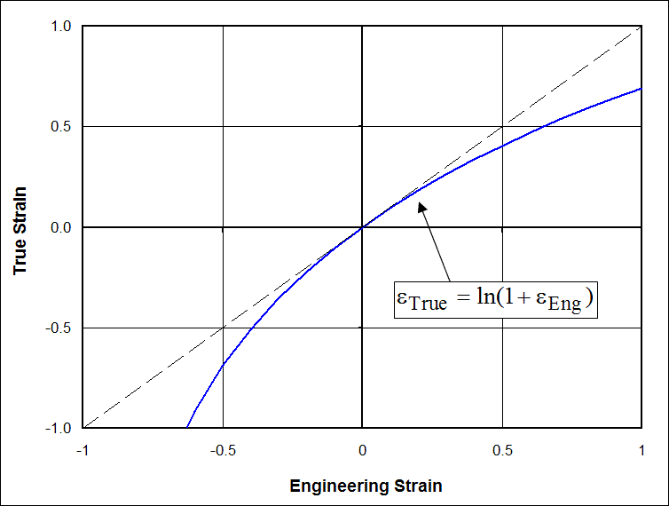
True Strain vs Engineering Strain
\[ \epsilon_{\text{True}} = \ln (1 + \epsilon_{\text{Eng}}) \]
because
\[ 1 + \epsilon_{\text{Eng}} \; \; = \; \; 1 + {\Delta L \over L_o} \; \; = \; \; {L_o \over L_o} + {\Delta L \over L_o} \; \; = \; \; {L_F \over L_o} \]
True Strain and Incompressible Materials
True strain possesses an additional property that is quite attractive when working with incompressible materials. To see this, recall this discussion on volume change on the hydrostatic and deviatoric strain webpage.
Recall that the ratio of initial to final volume is
\[ {V_F \over V_o} \, = \, \left( {W_F \over W_o} \right) \left( {D_F \over D_o} \right) \left( {H_F \over H_o} \right) \, = \, 1 \]
Now take the natural log of this equation to get
\[ \ln \left( {W_F \over W_o} \right) + \ln \left( {D_F \over D_o} \right) + \ln \left( {H_F \over H_o} \right) = 0 \]
But each log term is just the true strain. In fact, the sum is the trace of the true strain tensor.
\[ \epsilon^\text{True}_1 + \epsilon^\text{True}_2 + \epsilon^\text{True}_3 = 0 \qquad \text{(incompressible materials)} \]
Unlike small strains and Green strains, the above relationship applies to true strains even when the strains are finite.
Also, since the sum is zero, the rate of change of the sum will also always be zero for incompressible materials. So
\[ \dot \epsilon^\text{True}_1 + \dot \epsilon^\text{True}_2 + \dot \epsilon^\text{True}_3 = 0 \qquad \text{(incompressible materials)} \]
But since \(D = \dot \epsilon_{True}\), then the above equation can be written equally well as
\[ D_{11} + D_{22} + D_{33} = 0 \qquad \text{(incompressible materials)} \]
And furthermore, since each of these equations is the first invariant of its associated strain or rate of deformation tensor, the above identities are not limited to principal orientations and principal strains. They will apply even if shears are present.
True Strain and Volume Change
More generally, if the material is compressible, then the above relationship becomes\[ \ln \left( {V_F \over V_o} \right) \; = \; \ln \left( {W_F \over W_o} \right) + \ln \left( {D_F \over D_o} \right) + \ln \left( {H_F \over H_o} \right) \; = \; \epsilon^\text{True}_{\text{Vol}} \]
So
except this time, this applies for all strains, not just small ones.
Taking the time derivative again gives
\[ \dot \epsilon^\text{True}_1 + \dot \epsilon^\text{True}_2 + \dot \epsilon^\text{True}_3 = \dot \epsilon^\text{True}_{\text{Vol}} \]
and in terms of the rate of deformation tensor components...
\[ D_{11} + D_{22} + D_{33} = \dot \epsilon^\text{True}_{\text{Vol}} \]
Once again, this applies for finite strains, not just infinitesimal ones, and not just in principal orientations.
True Strain and Rotations
Things get complicated when the rate of deformation tensor is integrated over time to obtain true strain while rigid body rotations are present. Consider the following example of an object being stretched and rotated simultaneously.Tension Example with Rotation
In this example, the square starts out being stretched in the x-direction, but is also being rotated at the same time. It finishes after having rotated 90°, while all the time, being stretched in tension.
At \(t = 0\), the object is being stretched along the x-axis, and shrinking along the y-axis due to Poisson's effect. The rate of deformation tensor could be
\[ {\bf D} = \left[ \matrix{ 3.0 & \;\;\;0.0 \\ 0.0 & -2.0 } \right] \]
And if this takes place for 0.1 sec, then the integration of \(\int {\bf D}\,dt\) gives
\[ \boldsymbol{\epsilon}_{\text{True}} = \left[ \matrix{ 0.3 & \;\;\;0.0 \\ 0.0 & -0.2 } \right] \]
At some instant later, the object has rotated 45°, and continues to stretch. At this point, because it is at 45°, this deformation shows up as shear. So \({\bf D}\) could be
And if this occurs for another 0.1 sec, then the increment in true strain is
\[ \Delta \boldsymbol{\epsilon}_{\text{True}} = \left[ \matrix{ 0.00 & 0.15\\ 0.15 & 0.00 } \right] \]
and the total strain is the sum of the two.
\[ \boldsymbol{\epsilon}_{\text{True}} = \left[ \matrix{ 0.30 & \;\;\;0.15 \\ 0.15 & -0.20 } \right] \]
Then at a later time, the object has rotated 90° and is still being pulled in tension such that
\[ {\bf D} = \left[ \matrix{ -1.0 & 0.0 \\ \;\;\;0.0 & 1.5 } \right] \]
So the increment for this step is
\[ \Delta \boldsymbol{\epsilon}_{\text{True}} = \left[ \matrix{ -0.10 & 0.00\\ \;\;\;0.00 & 0.15 } \right] \]
Remember that it has been stretched to a longer length now, so \(dl/l\) is decreasing because the denominator is increasing.
Adding this to the previous total strain tensor gives
\[ \boldsymbol{\epsilon}_{\text{True}} = \left[ \matrix{ 0.20 & \;\;\;0.15 \\ 0.15 & -0.05 } \right] \]
The problem here is that the final true strain tensor is just a jumbled mess. It includes shear values, even though the corners remain at 90°, and ends with a negative \(D_{22}\) value even though the object was indeed stretching in the y-direction at the end of the process. This exemplifies the near uselessness of \(\int {\bf D}\,dt\) when rotations are present.
Tension Example with Rotations Again
This is the exact same example, but the strain state is calculated differently this time.At \(t = 0\), the object is being stretched along the x-axis, and shrinking along the y-axis due to Poisson's effect. The rate of deformation tensor is the same as before.
\[ {\bf D} = \left[ \matrix{ 3.0 & \;\;\;0.0 \\ 0.0 & -2.0 } \right] \]
And it takes place for 0.1 sec, and \({\bf R} = {\bf 0}\) at this point, so the integration of \(\int {\bf D}\,dt\) gives
\[ \boldsymbol{\epsilon}_{\text{True}} = \left[ \matrix{ 0.3 & \;\;\;0.0 \\ 0.0 & -0.2 } \right] \]
After the object has rotated 45°, \({\bf D}\) is now
\[ {\bf D} = \left[ \matrix{ 0.0 & 1.5 \\ 1.5 & 0.0 } \right] \]
But the rotation matrix is
\[ {\bf R} = \left[ \matrix{ 0.7071 & -0.7071 \\ 0.7071 & \;\;\;0.7071 } \right] \]
So \({\bf R}^T \cdot {\bf D} \cdot {\bf R}\) gives
\[ {\bf R}^T \cdot {\bf D} \cdot {\bf R} \; = \; \left[ \matrix{ 1.5 & \;\;\;0.0 \\ 0.0 & -1.5 } \right] \]
Multiplying this by 0.1 sec gives
\[ {\bf R}^T \cdot {\bf D} \cdot {\bf R}\,dt \; = \; \left[ \matrix{ 0.15 & \;\;\;0.0 \\ 0.0 & -0.15 } \right] \]
And adding this to the first result gives
\[ \boldsymbol{\epsilon}_{\text{True}} = \left[ \matrix{ 0.45 & \;\;\;0.00 \\ 0.00 & -0.35 } \right] \]
Finally, the object has rotated 90°. So \({\bf D}\) and \({\bf R}\) are
\[ {\bf D} = \left[ \matrix{ -1.0 & 0.0 \\ \;\;\;0.0 & 1.5 } \right] \qquad \qquad {\bf R} = \left[ \matrix{ 0 & -1 \\ 1 & \;\;\;0 } \right] \]
Computing \({\bf R}^T \cdot {\bf D} \cdot {\bf R}\) gives
\[ {\bf R}^T \cdot {\bf D} \cdot {\bf R} \; = \; \left[ \matrix{ 1.5 & \;\;\;0.0 \\ 0.0 & -1.0 } \right] \]
\[ {\bf R}^T \cdot {\bf D} \cdot {\bf R}\,dt \; = \; \left[ \matrix{ 0.15 & \;\;\;0.00 \\ 0.00 & -0.10 } \right] \]
And finally, adding this to the previous running total gives
\[ \boldsymbol{\epsilon}_{\text{True}} = \left[ \matrix{ 0.60 & \;\;\;0.00 \\ 0.00 & -0.45 } \right] \]
This result is much more intuitive. It shows that the object was stretched in its original x-direction and compressed in its original y-direction. And the components correspond to \(\ln (L_F / L_o)\), so they are still true strain type quantities.