Introduction
Vectors have magnitude and direction, and are used to represent physical quantities such as force, position, velocity, and acceleration. They are usually written in component form as \[ {\bf a} = ( 3, 7, 2 ) \] If the 3, 7, and 2 represent the x, y, and z components (or even r, \(\theta\), and z components) of some force, velocity, acceleration, etc, then they constitute a vector. If they instead represent the number of people who ate breakfast, lunch, and dinner with you, then they are not a vector. You get the idea.
A key question asked of a vector is, "Does it obey the usual rules of coordinate system transformations of vectors?" As expected, forces, accelerations, etc do. The number of people eating meals with you does not. Coordinate Transforms are discussed in detail here.
Where is the vector?
Does a vector contain information about its location? In general, no. In a force vector such as \( (3, 8, 5) \), the 3, 8, and 5 give the force component in each direction, but nothing about its position. A second position vector would be needed to specify the location of the force vector.Length of a Vector
The length of a vector is\[ |{\bf a}| = \sqrt{a^2_1 + a^2_2 + a^2_3} \]
Vector Length Example
If \( {\bf a} = ( 3, 7, 2 ) \), then\[ |{\bf a}| = \sqrt{3^2 + 7^2 + 2^2} = \sqrt{62} = 7.874 \]
Unit Vectors
A unit vector has a length equal to one. It is created by dividing each component of the vector by its total length.\[ {\bf u} = {{\bf a} \over |{\bf a}|} = {(a_1, a_2, a_3) \over \sqrt{a^2_1 + a^2_2 + a^2_3}} \]
Unit Vector Example
If \({\bf a} = ( 3, 7, 2 )\), then\[ {\bf u} = \left( {3 \over \sqrt{62}}, {7 \over \sqrt{62}}, {2 \over \sqrt{62}} \right) \]
Vector Addition
\[ (1, 3, 2) + (4, 1, 7) = (1+4, 3+1, 2+7) = (5, 4, 9) \]
Vector addition can be written as
\[ {\bf c} = {\bf a} + {\bf b} \quad \quad \quad \text{or} \quad \quad \quad c_i = a_i + b_i \]
The first form is vector or matrix notation, where non-scalars are written in bold font. The second form has many names: index, indicial, tensor, and Einstein notation.
Coordinate Systems
As simple as vector addition is, it does rely on one key rule that is often taken for granted. It is that both vectors must be in the same coordinate system. In fact, this is true for all vector and tensor operations.Dot Products
The dot product of two vectors is a scalar whose value is\[ {\bf a} \cdot {\bf b} = |{\bf a}| \, |{\bf b}| \cos \theta \]
where \(\theta\) is the angle between the two vectors. Applying this to the vector components gives
\[ \begin{eqnarray} {\bf a} \cdot {\bf b} & = & ( a_x {\bf i} + a_y {\bf j} + a_z {\bf k} ) \cdot( b_x {\bf i} + b_y {\bf j} + b_z {\bf k} ) \\ \\ & = & \matrix { a_x b_x ( {\bf i} \cdot {\bf i} ) & + & a_x b_y ( {\bf i} \cdot {\bf j} ) & + & a_x b_z ( {\bf i} \cdot {\bf k} ) & + \\ a_y b_x ( {\bf j} \cdot {\bf i} ) & + & a_y b_y ( {\bf j} \cdot {\bf j} ) & + & a_y b_z ( {\bf j} \cdot {\bf k} ) & + \\ a_z b_x ( {\bf k} \cdot {\bf i} ) & + & a_z b_y ( {\bf k} \cdot {\bf j} ) & + & a_z b_z ( {\bf k} \cdot {\bf k} ) } \\ \end{eqnarray} \]
but \( {\bf i} \cdot {\bf i} = {\bf j} \cdot {\bf j} = {\bf k} \cdot {\bf k} = 1 \) and \( {\bf i} \cdot {\bf j} = {\bf j} \cdot {\bf k} = {\bf k} \cdot {\bf i} = 0 \), leaving only
\[ {\bf a} \cdot {\bf b} = a_x b_x + a_y b_y + a_z b_z \]
Therefore, in summary, the dot product is
\[ {\bf a} \cdot {\bf b} = |{\bf a}| \, |{\bf b}| \cos \theta = a_x b_x + a_y b_y + a_z b_z \]
Dot Product Example
If \({\bf a} = ( 3, 7, 2 )\), and \({\bf b} = ( 1, 2, 3 )\), then\[ {\bf a} \cdot {\bf b} = 3 * 1 + 7 * 2 + 2 * 3 = 23 \]
and since \( |{\bf a}| = 7.874 \), and \( |{\bf b}| = 3.742 \), then \(\theta\) can be solved for to find that the angle between the vectors is 38.7°.
Dot Products and Unit Vectors
To find the length of \( {\bf a} \) in the direction of \( {\bf b} \), compute \( {\bf a} \cdot {\bf u_b} \) where \( {\bf u_b} \) is a unit vector in the direction of of \( {\bf b} \). To find the length of \( {\bf b} \) in the direction of \( {\bf a} \), compute \( {\bf b} \cdot {\bf u_a} \) where \( {\bf u_a} \) is a unit vector in the direction of of \( {\bf a} \).This works because the length of \( {\bf b} \) along the direction of \( {\bf a} \) is given by \(|{\bf b}| \cos \theta\), where \(\theta\) is the angle between the two vectors. But this is the same as \(|{\bf u_a}| |{\bf b}| \cos \theta\), since \(|{\bf u_a}| = 1\). So it is the same as \({\bf u_a} \cdot {\bf b}\).
Tensor Notation
A dot product is written in tensor notation simply as \( a_i b_i \). The summation from 1 to 3 is implied because the subscript ( \( i \) in this case ) appears twice ( on \( a \) and \( b \) ). In other words:Applications
Dot products are especially useful in calculating the work done by forces.\[ W = \int {\bf F} \cdot d{\bf x} \]
And yes, W can be a negative quantity. If you are in a tug-of-war and your \( \int {\bf F} \cdot d{\bf x} \) is negative, then you are losing.
The Sign of a Dot Product
The sign of a dot product is a very useful parameter for determining the relative orientation of two vectors. If the dot product equals zero, then the vectors are perpendicular to each other.If the dot product is negative, then the angle between the vectors is greater than 90°. If the two vectors happen to be forces, then a negative dot product implies that the forces are cancelling each other out to some degree because the angle between them is greater than 90°.
If the dot product is positive, then the angle between the vectors is less than 90° and the two are contributing constructively in a given direction.
Cross Products
\[ \begin{eqnarray} {\bf a} \times {\bf b} & = & ( a_x {\bf i} + a_y {\bf j} + a_z {\bf k} ) \times( b_x {\bf i} + b_y {\bf j} + b_z {\bf k} ) \\ \\ & = & \matrix { a_x b_x ( {\bf i} \times {\bf i} ) & + & a_x b_y ( {\bf i} \times {\bf j} ) & + & a_x b_z ( {\bf i} \times {\bf k} ) & + \\ a_y b_x ( {\bf j} \times {\bf i} ) & + & a_y b_y ( {\bf j} \times {\bf j} ) & + & a_y b_z ( {\bf j} \times {\bf k} ) & + \\ a_z b_x ( {\bf k} \times {\bf i} ) & + & a_z b_y ( {\bf k} \times {\bf j} ) & + & a_z b_z ( {\bf k} \times {\bf k} ) } \\ \end{eqnarray} \]
but \( {\bf i} \times {\bf j} = {\bf k} \) and \( {\bf j} \times {\bf k} = {\bf i} \) etc, while \( {\bf i} \times {\bf i} = {\bf j} \times {\bf j} = {\bf k} \times {\bf k} = 0 \), leaving
\[ {\bf a} \times {\bf b} = (a_y b_z - a_z b_y) {\bf i} + (a_z b_x - a_x b_z) {\bf j} + (a_x b_y - a_y b_x) {\bf k} \]
The result can be conveniently written as a determinant as follows
\[ {\bf a} \times {\bf b} = \left | \matrix { {\bf i\;} & {\bf j\;} & {\bf k\;} \\ a_x & a_y & a_z \\ b_x & b_y & b_z } \right | = (a_y b_z - a_z b_y) {\bf i} + (a_z b_x - a_x b_z) {\bf j} + (a_x b_y - a_y b_x) {\bf k} \]
The magnitude of a cross product is related to the sine of the angle between the two inputs.
\[ | {\bf a} \times {\bf b} | = |{\bf a}| \, |{\bf b}| \sin \theta \]
Tensor Notation
A cross product is written in tensor notation using the alternating tensor (also called the permutation tensor), \( \epsilon_{ijk} \), as follows\[ c_i = \epsilon_{ijk} a_j b_k \]
where \( \epsilon_{123} = \epsilon_{231} = \epsilon_{312} = 1 \), while \( \epsilon_{321} = \epsilon_{213} = \epsilon_{132} = -1 \), and all other combinations equal zero. Summation of the \(j\) and \(k\) indices from 1 to 3 is implied because they are repeated as subscripts in the above equation. In other words, it is shorthand for
\[ \matrix { c_i \; = \; \epsilon_{ijk} a_j b_k & = & \epsilon_{i11} a_1 b_1 & + & \epsilon_{i12} a_1 b_2 & + & \epsilon_{i13} a_1 b_3 & + & \\ & & \epsilon_{i21} a_2 b_1 & + & \epsilon_{i22} a_2 b_2 & + & \epsilon_{i23} a_2 b_3 & + & \\ & & \epsilon_{i31} a_3 b_1 & + & \epsilon_{i32} a_3 b_2 & + & \epsilon_{i33} a_3 b_3 } \]
The equation is still general until a particular component is chosen for \(i\) to be evaluated.
Cross Products Using Tensor Notation
Set \(i = 3\) to obtain the zth component of a cross product.\[ \matrix { c_3 \; = \; \epsilon_{3jk} a_j b_k & = & \epsilon_{311} a_1 b_1 & + & \epsilon_{312} a_1 b_2 & + & \epsilon_{313} a_1 b_3 & + & \\ & & \epsilon_{321} a_2 b_1 & + & \epsilon_{322} a_2 b_2 & + & \epsilon_{323} a_2 b_3 & + & \\ & & \epsilon_{331} a_3 b_1 & + & \epsilon_{332} a_3 b_2 & + & \epsilon_{333} a_3 b_3 } \]
All subscripts are now specified, and this permits evaluation of all alternating tensor components. All of them will equal zero except two. This leaves
\[ c_3 \; = \; \epsilon_{3jk} a_j b_k \; = \; a_1 b_2 - a_2 b_1 \]
which is consistent with the determinant result (as it had better be). Results for the xth and yth components are obtained by setting \(i\) equal to 1 and 2, respectively.
Applications
Cross products have applications in the areas of moments, rotations, and area calculations. The moment, \({\bf M}\), of a force is \({\bf r} \times {\bf F}\). This is written in tensor notation as\[ M_i = \epsilon_{ijk} r_j F_k \]
\[ v_i = \epsilon_{ijk} \omega_j r_k \]
And finally, the area of a triangle bounded on two sides by vectors \({\bf a}\) and \({\bf b}\) is
\[ Area = {1 \over 2} | \; {\bf a} \times {\bf b}| \]
In tensor notation, this is written in two steps as
\[ c_i = \epsilon_{ijk} a_j b_k \quad \quad \quad \text{and} \quad \quad \quad Area = {1 \over 2} \sqrt{c_i c_i} \]
or in a single equation as
\[ Area = {1 \over 2} \sqrt{ \epsilon_{ijk} a_j b_k \epsilon_{imn} a_m b_n } \]
Order of Factors in Tensor Notation
Tensor notation allows for increased flexibility of the order in which factors are written than is permitted in vector notation. For example, \( {\bf a} \times {\bf b} \) is not equal to \( {\bf b} \times {\bf a} \), although they are closely related. In contrast \( \epsilon_{ijk} a_j b_k \) equals \( \epsilon_{ijk} b_k a_j \) equals \( a_j b_k \epsilon_{ijk} \) because the order of operation is dictated by the indices rather than the order the factors are written in. So in the above discussion, \( \epsilon_{ijk} a_j b_k \epsilon_{imn} a_m b_n \) could also be written as \( \epsilon_{ijk} \epsilon_{imn} a_j b_k a_m b_n \). It is simply a matter of personal preference.Dyadic Products
Dyadic products seem to only arise in advanced mechanics applications, which is precisely what Finite Deformation Continuum Mechanics is, after all. A dyadic product of two vectors is a tensor (or matrix if you prefer). It is written as follows\[ \begin{eqnarray} {\bf a} \otimes {\bf b} & = & ( a_x {\bf i} + a_y {\bf j} + a_z {\bf k} ) \otimes( b_x {\bf i} + b_y {\bf j} + b_z {\bf k} ) \\ \\ \\ & = & \matrix { a_x b_x ( {\bf i} \otimes {\bf i} ) & + & a_x b_y ( {\bf i} \otimes {\bf j} ) & + & a_x b_z ( {\bf i} \otimes {\bf k} ) & + \\ a_y b_x ( {\bf j} \otimes {\bf i} ) & + & a_y b_y ( {\bf j} \otimes {\bf j} ) & + & a_y b_z ( {\bf j} \otimes {\bf k} ) & + \\ a_z b_x ( {\bf k} \otimes {\bf i} ) & + & a_z b_y ( {\bf k} \otimes {\bf j} ) & + & a_z b_z ( {\bf k} \otimes {\bf k} ) } \\ \\ \\ & = & \left[ \matrix { a_x b_x & a_x b_y & a_x b_z \\ a_y b_x & a_y b_y & a_y b_z \\ a_z b_x & a_z b_y & a_z b_z } \right] \\ \end{eqnarray} \]
In effect, the dyadic products such as \( ( {\bf i} \otimes {\bf i} ) \) and \( ( {\bf i} \otimes {\bf j} ) \) simply dictate the location of the terms in the tensor. A dyadic product is sometimes referred to as the outer product of vectors because of the following notation.
\[ {\bf C} \, = \, {\bf a} \otimes {\bf b} \, = \, \left\{ \! \matrix { a_x \\ a_y \\ a_z } \! \right\} \matrix { \{ b_x \quad b_y \quad b_z \} \\ \text{ } \\ \text{ } \\ } \, = \, \left[ \matrix { a_x b_x & a_x b_y & a_x b_z \\ a_y b_x & a_y b_y & a_y b_z \\ a_z b_x & a_z b_y & a_z b_z } \right] \]
Tensor Notation
Tensor notation of a dyadic product could not be simpler.\[ c_{ij} = a_i b_j \]
Dyadic products will be used in the calculation of resolved shear stresses on the traction vector page.
Dyadic Product Example
If \({\bf a} = ( 3, 7, 2 )\), and \({\bf b} = ( 1, 2, 3 )\), then\[ \begin{eqnarray} {\bf a} \otimes {\bf b} & = & \left[ \matrix { 3*1 & 3*2 & 3*3 \\ 7*1 & 7*2 & 7*3 \\ 2*1 & 2*2 & 2*3 } \right] \\ \\ \\ & = & \left[ \matrix { 3 & 6 & 9 \\ 7 & 14 & 21 \\ 2 & 4 & 6 } \right] \\ \end{eqnarray} \]
Miscellaneous
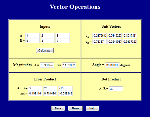
This webpage performs many vector operations. Try it out. Here's a screen shot.