Introduction
Classical dynamic material testing involves the application of a sinusoidal load to a sample and the recording of its displacement response. The load and displacement data are used to calculate stress and strain cycles. The ratio of the stress amplitude to the strain amplitude is the dynamic modulus. For shear loading, the usual symbol, \(G\), is used. The phase lag, \(\delta\), between the stress input and strain response is also recorded and usually presented as \(\tan(\delta)\). Various combinations of these parameters are plotted against strain amplitude, temperature, and/or frequency.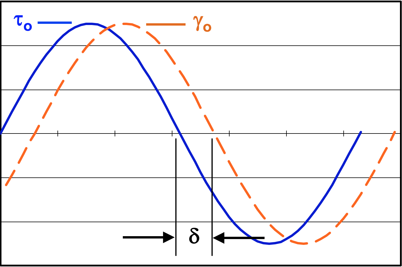
Definitions
\[ G^* = {\tau_o \over \gamma_o} \qquad \qquad J^* = {\gamma_o \over \tau_o} \]
Clearly \(G^* = 1 / J^*\) and vice-versa. The remaining fundamental quantity is the tangent of the phase lag, \(\tan(\delta)\), often simply called "tan delta" and sometimes called the "loss tangent".
The in-phase and out-of-phase components of the dynamic modulus are known as the storage modulus and loss modulus, respectively.
| Storage Modulus | \( \qquad G' = G^* \cos(\delta) \) |
| Loss Modulus | \( \qquad G'' = G^* \sin(\delta) \) |
From this, it is clear that \(\tan(\delta)\) is related to the ratio of \(G''\) to \(G'\).
\[ \tan(\delta) = {G'' \over G'} \]
The in-phase and out-of-phase components of the dynamic compliance are known as the storage compliance and loss compliance, respectively.
| Storage Compliance | \( \qquad J' = J^* \cos(\delta) \) |
| Loss Compliance | \( \qquad J'' = J^* \sin(\delta) \) |
And it is clear that \(\tan(\delta)\) is also related to the ratio of \(J''\) to \(J'\).
\[ \tan(\delta) = {J'' \over J'} \]
Incorrect Relationships
Do not be tempted to say that \(J' = 1 / G'\) and \(J'' = 1 / G''\), because these are incorrect. The correct relationships are\[ J' = J^* \cos(\delta) = { \cos(\delta) \over G^* } = { \cos^2(\delta) \over G' } \]
\[ J'' = J^* \sin(\delta) = { \sin(\delta) \over G^* } = { \sin^2(\delta) \over G'' } \]
It is perhaps easier to remember these as
\[ G' * J' = \cos^2(\delta) \qquad \quad \text{and} \qquad \quad G'' * J'' = \sin^2(\delta) \]
Strain Dependence
Here is some test data for a rubber sample. As with the uniaxial tension test data on the previous Mooney-Rivlin page, the stiffness of the rubber decreases as the strain amplitude increases. The curve labeled "GO" is for the portion of the test where the input load amplitude increases with time. The curve labeled "RETURN" is for the portion of the test where the input load amplitude decreases with time.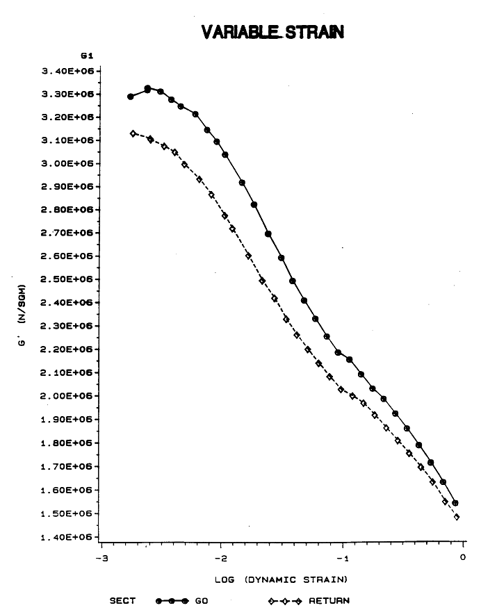
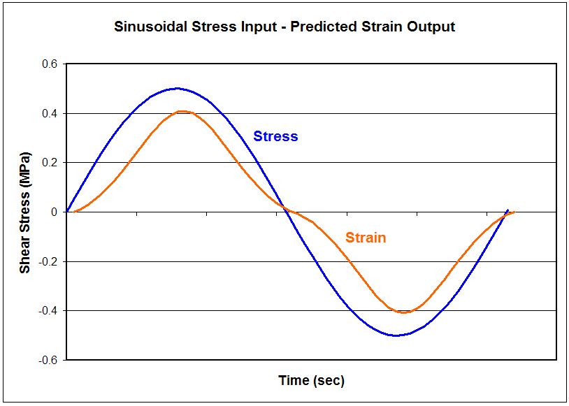
Below is a graph of the predicted shear strain for a sinusoidal shear stress input signal. The predictions are based on the material stiffness from the graph just above. Note how nonlinear the predicted shear strain is. In other words, the ratio of stress to strain as time passes is not constant (independent of the time delay due to the phase lag).
However, this is not the case for actual rubber behavior during dynamic tests. The actual strain signal is indistinguishable from the first figure at the top of this page.
Here is test data for the phase lag of the same rubber sample.

Temperature Dependence
This is a plot of \(J'\) and \(\tan(\delta)\) versus temperature.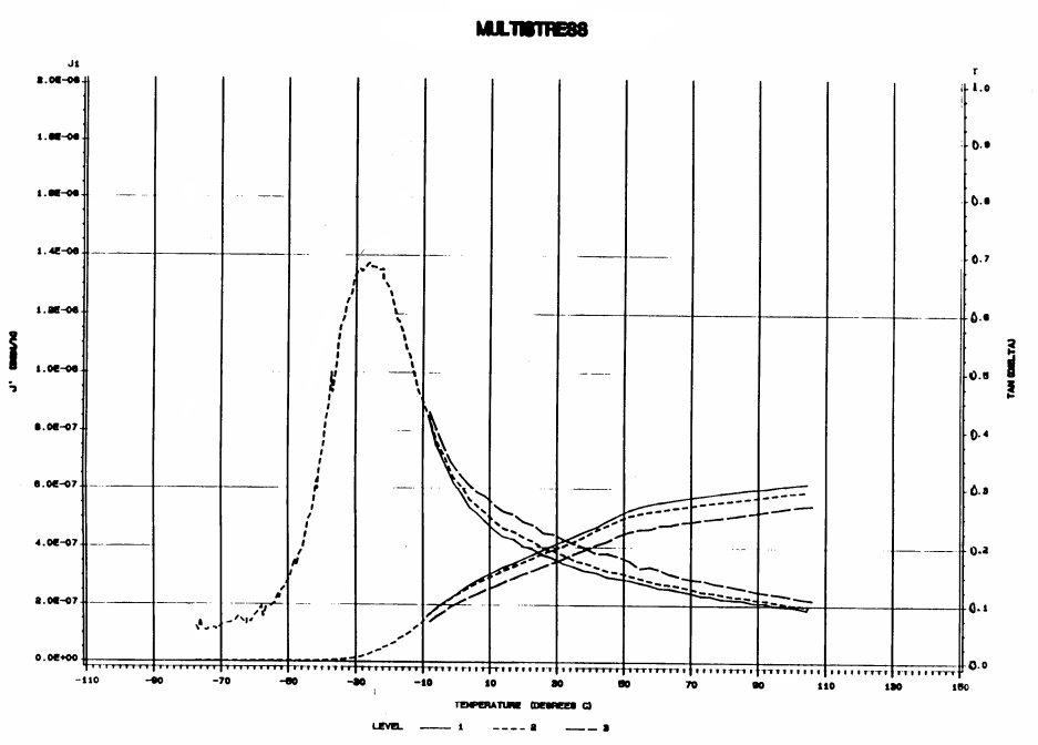
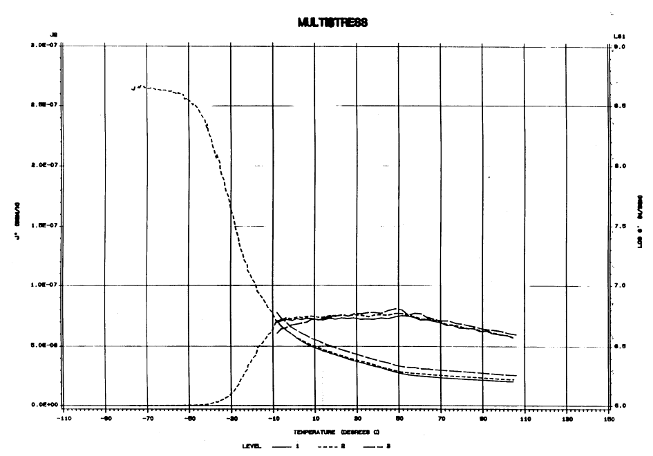
This is a plot of \(J''\) and \(\text{log}_{10}(G')\) versus temperature.
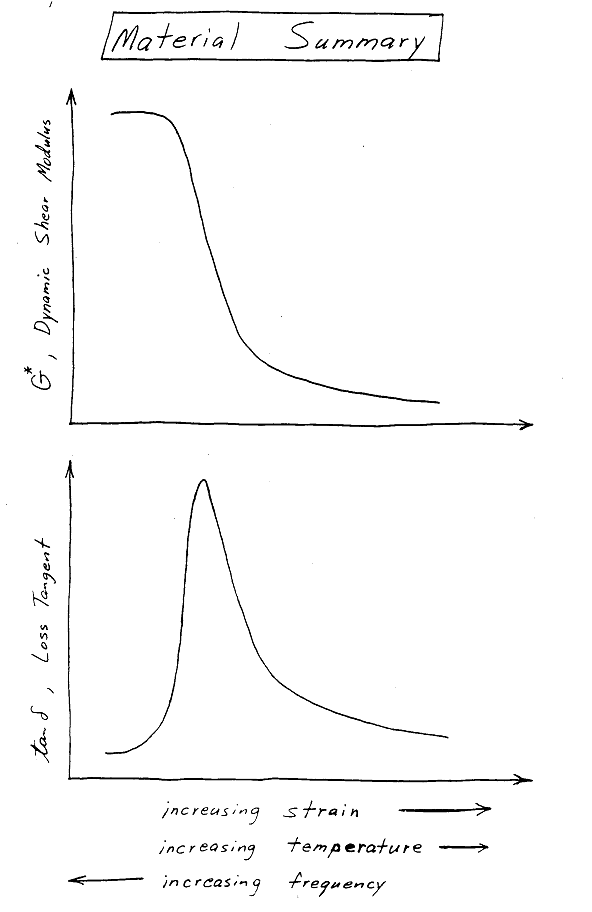
And here is a summary sketch. Note that temperature and frequency increase in opposite directions.
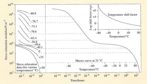
Time Temperature Equivalence
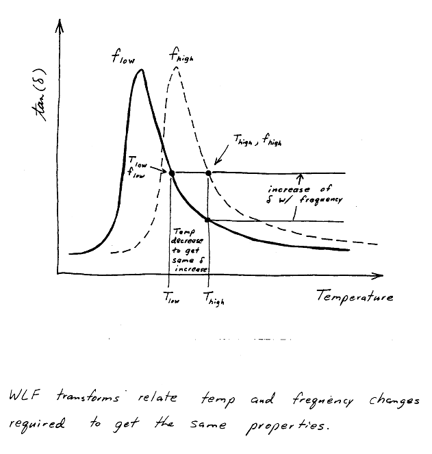
Around the time of World War II, Williams, Landel and Ferry reported a fascinating property of polymers: time-temperature equivalence. They observed that the dynamic material properties of a polymer at a reference temperature and frequency could be reproduced at a different combination of temperature and frequency that are related to the first pair by one simple equation. That equation is now known as the WLF Equation or WLF Transform.Time-temperature equivalence means that the stiffness and hysteresis of a polymer will be the same at the proper combination of low temperature and low frequency as at a given combination of high temperature and high frequency.
This property is very beneficial from an experimental viewpoint because it means that the viscoelastic properties of materials at thousands of Hertz can be estimated in the lab by testing at low frequencies and very low temperatures. (This is often done for traction studies.)
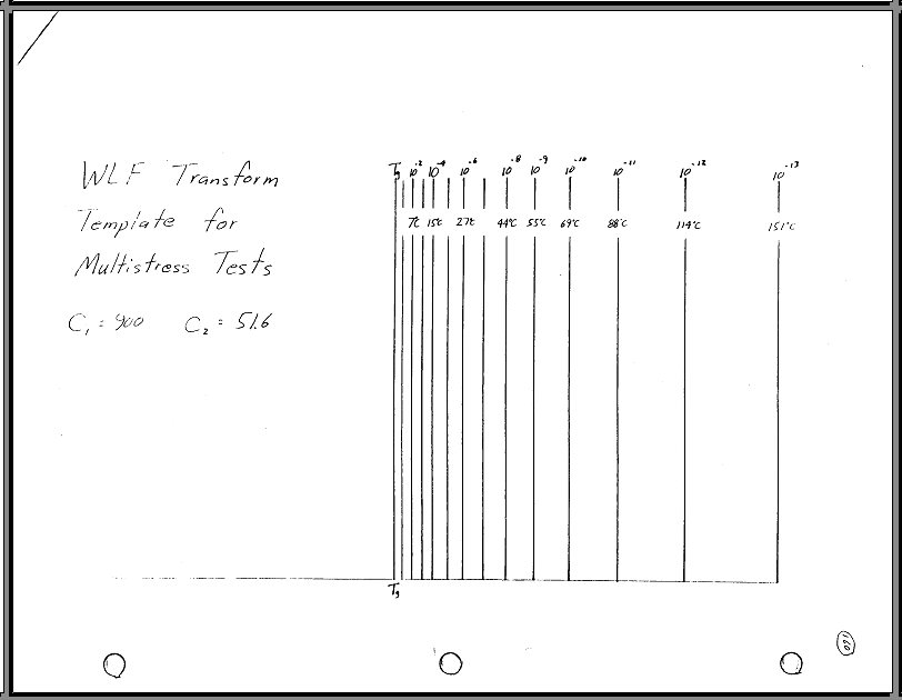
WLF Transforms
\[ \log_{10} \left( {f_1 \over f_0} \right) = {-C_1 (\theta_1 - \theta_0) \over (C_2 + \theta_0) (C_2 + \theta_1) } \]
where:
\(\theta_0 = T_0 - T_g\) \(\theta_1 = T_1 - T_g\)
Usual values of the constants are \(C_1\) = 900 and \(C_2\) = 51.6 .
The coefficients, \(C_1\) and \(C_2\), are obtained by curve fitting the WLF equation to experiemental data. They change little regardless of the application. For example, estimates from test in MFG on PL KM's gave \(C_1 = 900\) and \(C_2 = 55\). But it must be noted that there was a great deal of uncertainty in these estimates.
Overall, the WLF transform is considered to perform quite well, though not perfectly, over many decades of frequency and at \(T_g\) ≤ \(T\) ≤ \(T_g\)+100°C. The WLF transform can be rearranged to solve for \(\theta_1\), which is more useful.
\[ T_1 - T_g = { C_1 \theta_0 - C_2 ( C_2 + \theta_0 ) \log_{10} ( f_1 / f_0 ) \over C_1 + ( C_2 + \theta_0 ) \log_{10} ( f_1 / f_0 ) } \]
WLF Example
Consider the multistress test results above. The graph gives the material properties at 10 Hz over a wide range of temperatures. Let's (arbitrarily) start with \(\tan(\delta)\) at 10 Hz, 70°C, and at the 0.035 kg/mm2 stress level, (the long-dashed curve on the graph). At these conditions, \(\tan \delta\) = 0.17 . To estimate \(\tan \delta\) at 70°C and 100 Hz, use\[ \begin{eqnarray} C_1 & = & 900 \qquad & T_0 & = & 70^\circ\text{C} \\ C_2 & = & 51.6 \qquad & f_0 & = & 10 \text{ Hz} \\ T_g & = & \text{-}20^\circ\text{C} \qquad & f_1 & = & 100 \text{ Hz} \end{eqnarray} \]
to get \(T_1\) = 51°C. At 51°C and 10 Hz, \(\tan \delta\) = 0.2 . Therefore, at \(T_1\) = 70°C and 100 Hz, \(\tan \delta\) should also equal 0.2.
More extensive experimental data looks like this.