Strain Gauges

Introduction

Ref: http://www.doitpoms.ac.uk/tlplib/mechanical-testing/notes.php

Strain gauges measure strain on the surface of objects. They do so by changing their electrical resistance as they stretch with the objects they are glued to. The resistance change is proportional to the amount of stretching they experience and is reflected as a change in voltage across designated elements, one being the strain gauge itself, in an electrical circuit.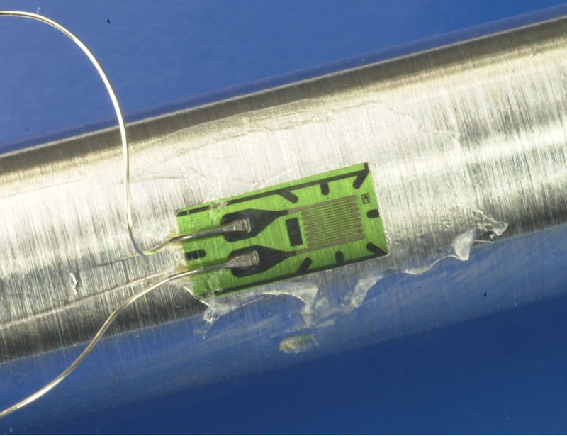

The photo at the right shows a strain gauge mounted on a tube. Note that it is aligned to measure strains along the length of the tube, not around it. This is evident by the directional nature of the gauge in its right half. It contains a single continuous wire running back and forth, longitudinally along the tube. The left half contains the electrical leads with wires leading to the rest of the electrical circuit.

This page will discuss the fundamental physics governing strain gauges, how they are used in electrical circuits to maximize measurement sensitivity, and how they are used in combinations such as rosettes and to isolate bending and shear.

Gauge or Gage

The two words are used interchangeably, and both appear in reports and on websites. If Vishay, a world leader in strain gauge production is to be believed, "gage" is the American spelling, and "gauge" is the British spelling.

A Google search for "strain gauge" returns nearly six times as many hits as "strain gage", 9,500,000 versus 1,700,000. And Wikipedia contains a "Strain Gauge" page, but not one for "Strain Gage".

I've used "gauge" here due to its overwhelming popularity according to Google.

Fundamental Concepts

Strain gauges measure strain in only one direction. In the sketch at the right, that direction is horizontal because it is the orientation of the fine wire that zig-zags back and forth. Because they measure strain in only one direction, a single strain gauge is often referred to as an axial gauge, which is short for uniaxial gauge, a name reflecting its sensitivity to strain in only one direction.

The sketch shows the key components of a strain gauge. Chief among these is the active grid section. As can be seen, this area contains a single continuous wire whose resistance changes as the gauge is stretched.

The wire's electrical resistance, \(R\), is related to its length, \(L\), and area, \(A\), by

\[ R = {\rho \; L \over A} \]
where \(\rho\) is resistivity, an electrical property of the wire's material. For copper, \(\rho = 1.7*10^{-8} \Omega \text{m}\). As the wire is stretched, its length increases while its cross-sectional area decreases due to Poisson effects. As can be seen in the equation, both of these changes cause the wire's resistance to increase. Likewise, compression will cause the wire's resistance to decrease.

The wire's resistance change is related to strain by way of the so-called Gauge Factor, \(GF,\) which is defined as

\[ GF \; = \; {\Delta R / R \over \Delta L / L} \; = \; {\Delta R / R \over \epsilon} \]
The terms \(\Delta R/R\) and \(\Delta L/L\) represent percentage changes in resistance and wire length, respectively. The gauge factor is simply the ratio of these percentage changes, with the length term corresponding to mechanical strain. Therefore, the strain gauge's change in resistance, as a function of strain, is

\[ \Delta R = R * GF * \epsilon \]
Gauge factor values are approximately 2, though they can stray from this by several percent. The example below explains why.

Theoretical Gauge Factor Values

It turns out that gauge factors can be estimated from the \(R = \rho L / A\) relationship by first determining \(dR/dL\) as follows

\[ \begin{eqnarray} {dR \over dL} & = & {\partial R \over \partial L} + \left( {\partial R \over \partial A} \right) \left( {dA \over dL} \right)\\ \\ & = & {\rho \over A} + \left( {-\rho L \over A^2} \right) \left( {-A \over L} \right)\\ \\ & = & 2 {\rho \over A} \end{eqnarray} \]
and then multiplying through by \(L / R\). (The \(dA/dL\) term above will be explained in a moment.)

\[ GF \quad = \quad {dR \over dL} * {L \over R} \quad = \quad \left( 2 {\rho \over A} \right) \left( {L \over \left( {\rho L \over A} \right) } \right) \quad = \quad 2 \]
This results in a theoretical value of 2 for all gauge factors, independent of wire material, length, and cross-section. (Recall that actual gauge factors usually vary from this by several percent.)

A key step in this derivation was the assignment of \(dA/dL\) to \((\text{-}A/L)\). This carries with it an assumption that the wire maintains constant volume as it stretches. In other words, \(L*A = const\). Taking differentials of this produces \(d(L*A) = L*dA + A*dL = 0\), which can be rearranged to give

\[ {dA \over dL} = - {A \over L} \]
It is curious that an incompressible assumption, which is usually associated with plastic deformation, can lead to a close approximation of \(GF\) even when the gauges themselves are operated in the linear elastic regime.

Strain Gauge Sensitivity

We've seen that a strain gauge's resistance changes with strain according to \(\Delta R = R*GF*\epsilon\). But what we haven't yet discussed is that this resistance change is in fact a very small fraction of the gauge's nominal resistance, and that this presents major challenges to the goal of measuring strain.

To see this, plug some values into the equation. For example, take \(R = 350 \, \Omega\), \(GF = 2\), and \(\epsilon = 0.0001\). The \(350 \, \Omega\) resistance is a typical value for a strain gauge, and \(\epsilon = 0.0001\) is a typical strain level for metallic objects. It corresponds to about 7 MPa (~1,000 psi) in aluminum and about 20 MPa (~3,000 psi) in steel.

These values give

\[ \begin{eqnarray} \Delta R & = & R * GF * \epsilon\\ \\ & = & (350 \, \Omega)(2)(0.0001)\\ \\ & = & 0.07 \, \Omega \end{eqnarray} \]
This resistance change of \(0.07 \, \Omega\) is only 0.02% of the gauge's resistance. This challenges technology to discern such small percentages. The resolution to this challenge is the Wheatstone Bridge Circuit... discussed next.

Electrical Circuits - Wheatstone Bridge

The electrical circuit containing the strain gauge is as important as the gauge itself. It is the job of the electrical circuit to relate the change in the gauge's resistance to a measurable change in voltage. The Wheatstone Bridge circuit shown at the right is by far the most popular choice for accomplishing this. It is also called a quarter bridge circuit because the gauge itself is one of four resistances in the circuit.

The feature of this circuit that makes it so popular is its ability to convert a small change in resistance into a measurable voltage differential. Recall the strain gauge sensitivity example just above in which the resistance of the gauge changed \(0.07 \, \Omega\) out of \(350 \, \Omega\), or only 0.02%. In contrast, although the variation of \(V_{meas}\) in a Wheatstone Bridge circuit is also small, it varies about zero instead of a large offset value as the strain gauge resistance does. In fact, it will be shown below that \(V_{meas}\) is proportional to \(\epsilon\). So the change in \(V_{meas}\) on a percentage basis is large.

Wheatstone Bridge Circuit Analysis

Analysis of the Wheatstone Bridge circuit is straightforward, but even so, it can initially seem daunting because of the diamond shape in the circuit as shown above. Hence, the figure at the right is provided to lay-out the circuit in a more familiar, and electrically equivalent orientation. Recall that the ultimate goal is to determine \(V_{meas}\), which is \(V_g - V_3\). The analysis proceeds as follows.

Begin by determining the currents, \(I_1\) and \(I_2\), flowing through each leg of the circuit.

\[ I_1 = {V_{in} \over R_1 + R_3} \qquad \qquad I_2 = {V_{in} \over R_2 + R_G} \]
The voltages just above \(R_3\) and \(R_G\) are

\[ V_3 = I_1 R_3 \qquad \qquad V_g = I_2 R_G \]
Substituting for \(I_1\) and \(I_2\) gives

\[ V_3 = V_{in} {R_3 \over R_1 + R_3} \qquad \qquad V_G = V_{in} {R_G \over R_2 + R_G} \]
And finally, subtracting \(V_3\) from \(V_g\) gives \(V_{meas}\).

\[ V_{meas} = V_{in} \left[ {R_G \over R_2 + R_G} - {R_3 \over R_1 + R_3} \right] \]
This is the fundamental relationship from which everything else procedes. As an example, consider the simplest scenario of choosing resistors such that \(R_1\), \(R_2\), and \(R_3\) all equal \(R_{G,o}\), the strain gauge's resistance at zero strain. It should be clear that \(V_{meas} = 0\) when all four resistances are equal. In this case, the bridge is said to be balanced.

But recall that the gauge's resistance, \(R_G\), changes with strain. This will lead to nonzero values of \(V_{meas}\). This achieves the desired result of having \(V_{meas} = 0\) when \(\epsilon = 0\) and \(V_{meas}\) changing values when \(\epsilon\) does.

There are many, many variations on this basic arrangement. They will be discussed below.

Let's rewrite the basic Wheatstone Bridge circuit equation for reference here since it is so important.

\[ V_{meas} = V_{in} \left[ {R_G \over R_2 + R_G} - {R_3 \over R_1 + R_3} \right] \]
This equation is just messy enough that it is difficult to see the influence of \(R_G\) on \(V_{meas}\). So let's simplify it. Begin by expressing the gauge's resistance, \(R_G\), as the sum of its nominal zero-strain value, \(R_{G,o}\), plus its change due to strain, \( \Delta R_G\).

\[ R_G = R_{G,o} + \Delta R_G \]
Replacing \(R_G\) with this gives

\[ V_{meas} = V_{in} \left[ {R_{G,o} + \Delta R_G \over R_2 + R_{G,o} + \Delta R_G} - {R_3 \over R_1 + R_3} \right] \]
And for the simplest scenario, select resistors \(R_1, R_2,\) and \(R_3\) to be equal to \(R_{G,o}\).

\[ V_{meas} = V_{in} \left[ {R_{G,o} + \Delta R_G \over 2 R_{G,o} + \Delta R_G} - {1 \over 2} \right] \]
And apply some algebra to simplify the expression to

\[ V_{meas} = V_{in} \left[ {\Delta R_G \over 4 R_{G,o} + 2 \Delta R_G} \right] \]
Now it's time to once again recall that \(\Delta R\) is a tiny fraction of \(R_{G,o}\). The \(\Delta R\) term can therefore be dropped from the denominator of the equation. This leaves

\[ V_{meas} = V_{in} \left[ {1 \over 4 R_{G,o}} \right] \Delta R_G \]
This is a very helpful expression. It reveals that the Wheatstone Bridge circuit accomplishes the desired goal of producing a voltage, \(V_{meas}\), that is proportional to \(\Delta R\), and therefore proportional to strain. To see this more directly, recall that \(\Delta R_G = R_{G,o} * GF * \epsilon\) and substitute.

\[ V_{meas} = V_{in} \left[ {1 \over 4 R_{G,o}} \right] R_{G,o} * GF * \epsilon \]
Solving for strain gives

\[ \epsilon = \left( {4 \over GF} \right) \left( { V_{meas} \over V_{in} } \right) \]
It is tempting to conclude from this that only the gauge's gauge factor, \(GF\), and the circuit's excitation voltage, \(V_{in}\), are needed to convert measured voltages, \(V_{meas}\), to strains. But recall that the derivation also required that we select resistors satisfying \(R_1 = R_2 = R_3 = R_{G,o}\). So it is also necessary to know the nominal resistance of the strain gauge.

Practical Considerations - Thermal Heating

On a practical note, an experimentalist dealing with the very real-world issues of measurement uncertainties and signal-to-noise ratios might conclude from the above equation that one should use the largest excitation voltage, \(V_{in}\), possible in order to produce the largest measured voltages possible, thereby maximizing measurement sensitivity. And this is generally true.

But there is a practical consideration that limits \(V_{in}\). It is that large voltages, which naturally lead to large currents, can produce high heat generation rates (which any good engineer should reflexively recognize as something to be avoided even before he knows why!).

In this case, high heat generation rates can cause problems for the electronics in the data acquisition system. Specifically, as things heat up, they expand. The key consequence is that the resistance of the strain gauges in the Wheatstone Bridge circuit can and will change. This is obviously bad because it leads to nonzero \(V_{meas}\) even though \(\epsilon = 0\). Worse, the heat generated by the strain gauge can pass into the object it is attached to and heat it, causing it to expand. This will show up as measured strain, even though it is not caused by any loads. This scenario can be worse in composites than in metals because metals are usually good heat conductors and can therefore conduct the heat generated in the strain gauge away with minimal temperature rise.

In practice, \(V_{in}\) varies from 2 Volts to 10 Volts. This range is a compromise between the desire to maximize the excitation voltage in order to maximize measurement sensitivity, and the competing desire to minimize heat generation in the system.

Balancing a Wheatstone Bridge

We talked just above about scenarios that can lead to nonzero strain measurements in the presence of what-is-in-fact zero strain because of deviations of the resistors, and the gauge itself, from their nominal resistances, usually due to temperature changes. This can come from heat generation in the electronics as well as changes in the ambient temperature. When this occurs, the bridge circuit is said to be unbalanced. It is a common problem. The solution is to introduce a variable resistor in place of one of the three in the circuit, and to tune it until \(V_{meas} = 0\). We can see how this works.

Once again, rewrite the basic Wheatstone Bridge circuit equation for reference because it is the starting point.

\[ V_{meas} = V_{in} \left[ {R_G \over R_2 + R_G} - {R_3 \over R_1 + R_3} \right] \]
Set \(V_{meas} = 0\) and solve the remaining expression for the resistances.

\[ {R_G \over R_2 + R_G} - {R_3 \over R_1 + R_3} = 0 \]
Simplifying gives

\[ R_1 R_G = R_2 R_3 \]
In general, one of the three resistors in a Wheatstone bridge circuit will be adjustable. Its resistance can be tuned until the above equation is satisfied, thereby producing zero measured voltage at zero strain, at least for that moment. It is still possible that the ambiant temperature may change during the test and produce misleading results. Such scenarios will be discussed farther down the page.

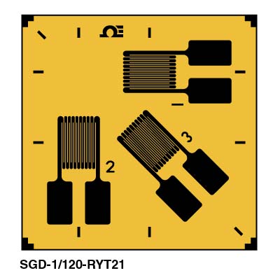
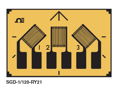
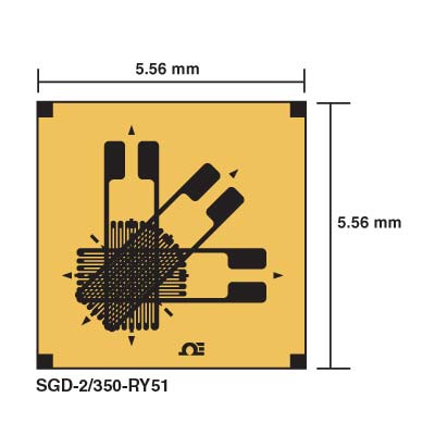
Strain Gauge Rosettes

A strain gauge rosette is simply three conventional axial gauges placed close together and at prescribed orientations relative to each other. Three sample rosettes are shown below. Each rosette here contains gauges at 45° relative orientations, although 60° relative orientations are also available. Note that each gauge in a rosette is independent of the others, with each gauge having its own Wheatstone bridge circuit.

The key feature of a strain gauge rosette is its ability to determine the complete strain state on the surface of an object. This includes all normal and shear strains, as well as principal strains and the principal orientation. This capability is explained next.

Ref: http://www.omega.com/

2-D coordinate transformations of the strain tensor are the key to understanding strain gauge rosettes. In particular, this equation giving the normal strain at any orientation, \(\theta\), is exploited by rosettes.

\[ \epsilon'\!_{xx} = \epsilon_{xx} \cos^2 \theta + \epsilon_{yy} \, \sin^2 \theta + 2 \left( {\gamma_{xy} \over 2} \right) \sin \theta \cos \theta \]
The key concept is to let \(\epsilon_{xx}\), \(\epsilon_{yy}\), and \(\gamma_{xy}\) be the unknown strain state that is to be determined, and let three separate \(\epsilon'\!_{xx}\) values be the strain values read by the three strain gauges in the rosette. The strains read by the gauges at 0°, 45°, and 90° will be called \(\epsilon_{0^\circ}\), \(\epsilon_{45^\circ}\), and \(\epsilon_{90^\circ}\), respectively.

Note that you are free to choose any direction to be the x-axis, and then align the 0° rosette gauge with that direction. It is recommended to choose the length direction of a bar or beam to be the 0° x-axis direction as this usually simplifies subsequent calculations.

Two-thirds of the problem is easily solved by simply aligning the rosette such that 0° corresponds to the x-axis and 90° corresponds to the y-axis. This gives \(\epsilon_{xx} = \epsilon_{0^\circ}\) and \(\epsilon_{yy} = \epsilon_{90^\circ}\).

This leaves only \(\gamma_{xy}\) remaining to be determined. This is accomplished by selecting \(\theta = 45^\circ\) and inserting into the equation to obtain.

\[ \epsilon_{45^\circ} = \epsilon_{xx} \cos^2 45^\circ + \epsilon_{yy} \, \sin^2 45^\circ + 2 \left( {\gamma_{xy} \over 2} \right) \sin 45^\circ \cos 45^\circ \]
But \(\epsilon_{xx} = \epsilon_{0^\circ}\), \(\; \epsilon_{yy} = \epsilon_{90^\circ}\), and \(\; \sin 45^\circ = \cos 45^\circ = 1 / \sqrt{2}\). Insert these to get

\[ \epsilon_{45^\circ} = { \epsilon_{0^\circ} + \epsilon_{90^\circ} + \gamma_{xy} \over 2 } \]
and solve for \(\gamma_{xy}\)

\[ \gamma_{xy} = 2 \epsilon_{45^\circ} - \epsilon_{0^\circ} - \epsilon_{90^\circ} \]
This gives the complete 2-D strain state on the surface of an object.

And if desired, the principal strains can then be determined from the basic strain components using the usual relationship, which is given here for completeness.

\[ \epsilon_{max}, \epsilon_{min} = {\epsilon_{xx} + \epsilon_{yy} \over 2} \pm \sqrt{ \left( {\epsilon_{xx} - \epsilon_{yy} \over 2} \right)^2 + \left( \gamma_{xy} \over 2 \right)^2 } \]
And the principal orientation, \(\theta_P\), is given by

\[ \tan (2 \theta_P) \; = \; {\gamma_{xy} \over \epsilon_{xx} - \epsilon_{yy} } \]

Strain Gauge Rosette Example

What are the principal strains at a point if a strain gauge rosette reads: \(\epsilon_{0^\circ} = 0.02\), \(\; \epsilon_{45^\circ} = 0.03\), and \(\; \epsilon_{90^\circ} = 0.05 \; \)?

\(\epsilon_{xx}\) and \(\epsilon_{yy}\) are the easy ones.

\[ \epsilon_{xx} = \epsilon_{0^\circ} = 0.02 \qquad \qquad \epsilon_{yy} = \epsilon_{90^\circ} = 0.05 \]
And the shear strain, \(\gamma_{xy}\), is

\[ \begin{eqnarray} \gamma_{xy} & = & 2 \, \epsilon_{45^\circ} - \epsilon_{0^\circ} - \epsilon_{90^\circ} \\ \\ & = & 2 * 0.03 - 0.02 - 0.05 \\ \\ & = & \text{-}\,0.01 \end{eqnarray} \]
The principal strains are

\[ \begin{eqnarray} \epsilon_{max}, \epsilon_{min} & = & {\epsilon_{xx} + \epsilon_{yy} \over 2} \pm \sqrt{ \left( {\epsilon_{xx} - \epsilon_{yy} \over 2} \right)^2 + \left( \gamma_{xy} \over 2 \right)^2 } \\ \\ \\ & = & {0.02 + 0.05 \over 2} \pm \sqrt{ \left( {0.02 - 0.05 \over 2} \right)^2 + \left( \text{-}\,0.01 \over 2 \right)^2 } \\ \\ \\ & = & 0.053, \, 0.017 \end{eqnarray} \]

Strain Gauge Placement

Ref: http://www.americanrifle.com/

One might think that a strain gauge can be placed at any desired location on an object to measure strain. And while it may be true that a gauge can indeed be placed at most any location, that does not mean that it is always possible to obtain an accurate, reliable measure of strain from any location.

The key issue is that gauges have a finite size, often several millimeters, and they basically average the strain measurement under their "footprint". This is fine when strains don't vary appreciably with position. But means that reliable strain measures are effectively impossible in regions with high strain gradients. These inevitably occur at stress concentrations, such as holes, fillets, notches, etc, as shown at the right. These are often the very places at which strain measurements are most desired. Although a gauge placed in a fillet will report a strain value, it should not be trusted.

This issue cannot be overcome with the strain gauge alone. The usual plan-of-attack is to place the gauge at a location removed from the concentration, where it is anticipated that the strain level will be significant (in order to maximize signal-to-noise), but not on a high gradient. In the picture here, such locations are green. Finite element methods would then be used to predict the stress levels in the fillets, and the accuracy of their predictions would be judged based on how well they match the strain gauge readings in the nearby, low-gradient areas.

In addition to the challenges of placement location, there is also the issue of placement orientation uncertainty and error. As with many aspects of strain gauge analysis, the effects of misorientation are best analyzed via the 2-D coordinate transform equation for normal strain.

\[ \epsilon'\!_{xx} = \epsilon_{xx} \cos^2 \theta + \epsilon_{yy} \, \sin^2 \theta + 2 \left( {\gamma_{xy} \over 2} \right) \sin \theta \cos \theta \]
In this case, \(\epsilon'\!_{xx}\) is the normal strain measured by the strain gauge at some misorientation angle, \(\theta\), \(\; \epsilon_{xx}\) is the value that the gauge would measure if it were properly aligned, i.e., at \(\theta = 0^\circ\), \(\; \epsilon_{yy}\) is the strain normal to the local x-direction, and \(\gamma_{xy}\) is the shear strain.

Strain Gauge Misalignment Example

As an example, a misalignment angle of 6° gives an interesting relationship that is easy to remember.

\[ \begin{eqnarray} \epsilon'\!_{xx} & = & \epsilon_{xx} \cos^2 6^\circ + \epsilon_{yy} \, \sin^2 6^\circ + 2 \left( {\gamma_{xy} \over 2} \right) \sin 6^\circ \cos 6^\circ \\ \\ & = & 0.99 \, \epsilon_{xx} + 0.01 \, \epsilon_{yy} + 0.10 \, \gamma_{xy} \end{eqnarray} \]
This shows that at a misalignment angle of 6°, the strain gauge will report

99% of the strain in the direction that the gauge was supposed to have been placed,
1% of the strain perpendicular to the intended direction, and
10% of the shear strain present

Even at the relatively large misalignment angle of 6°, a strain gauge can still report accurate values if shear strains are small. But if \(\gamma_{xy}\) is large, then the gauge reading will be polluted by 10% of the shear strain value.

Another consideration is that while only a tiny fraction of \(\epsilon_{yy}\) will bleed into the reported value, this can still be significant if \(\epsilon_{yy}\) is much larger than \(\epsilon_{xx}\). However, if this is indeed the case, then the gauge probably should have been aligned in the y-direction in the first place to maximize the measured signal.

Isolating Temperature - Half Bridge

Perhaps the simplest method of eliminating temperature effects is to mount a strain gauge on a piece of structure that is not loaded and does not deform. Then any strain reported by this gauge can be assumed to be entirely due to thermal drift, and this strain can be subtracted from nearby gauge readings. This assumes that all gauges are subjected to the same temperatures, and that they all respond to temperature variations similarly (usually not a bad assumption, in fact).

An alternative approach is the so-called half-bridge circuit shown here. In this case, a second gauge is wired into the circuit as shown. As above, this second gauge is also mounted on unloaded structure nearby the primary strain-measuring gauge so that both gauges will experience the same operating temperatures. Analysis of this circuit follows...

As always, start with the fundamental equation for voltages in a Wheatstone Bridge circuit.

\[ V_{meas} = V_{in} \left[ {R_G \over R_2 + R_G} - {R_3 \over R_1 + R_3} \right] \]
Recall that in earlier analyses, the strain gauge resistance was expressed as \(R_G = R_{G,o} + \Delta R_G\), where \(R_{G,o}\) is the nominal resistance of the gauge at the reference temperature and when unloaded, and \(\Delta R_G\) is the change in the gauge's resistance.

Now, further partition \(\Delta R_G\) as follows

\[ R_G = R_{G,o} + \Delta R_\theta + \Delta R_\epsilon \]
where \(\Delta R_\theta\) is the change in the gauge's resistance due to temperature changes (the unwanted part), and \(\Delta R_\epsilon\) is the change in its resistance due to strain. Note that the "temp gauge" will not experience any strain, so \(\Delta R_\epsilon = 0\) for it. Also, since both gauges are mounted near each other, \(\Delta R_\theta\) will be the same for both. This gives

\[ \begin{eqnarray} R_{G2} & = & R_{G,o} + \Delta R_\theta \\ \\ R_{G1} & = & R_{G,o} + \Delta R_\theta + \Delta R_\epsilon \end{eqnarray} \]
Substituting these relationships into the basic equation, and setting \(R_1 = R_3 = R_{G,o}\) gives (after much algebra)

\[ V_{meas} = V_{in} \left[ {\Delta R_\epsilon \over 4 R_{G,o} + 2 \Delta R_\theta + 2 \Delta R_\epsilon} \right] \]
Once again, the changes in resistance, \(\Delta R_\theta\) and \(\Delta R_\epsilon\), will be much less than \(R_{G,o}\) and can be neglected in the denominator. This again leaves

\[ V_{meas} = V_{in} \left[ {\Delta R_\epsilon \over 4 R_{G,o} } \right] \quad \qquad \text{and} \qquad \quad \epsilon = \left( {4 \over GF} \right) \left( { V_{meas} \over V_{in} } \right) \]
as before. But the very important change now is that temperature effects are completely eliminated (assuming both gauges experience the same temperatures).

Note that the reference "temp gauge" must be wired into the same leg of the Wheatstone bridge as the main strain gauge for this to work!

Isolating Shear - Full Bridge

Shear can be isolated and measured by using a strain gauge in place of every resistor in a Wheatstone Bridge circuit. For such applications, the four gauges come in a unit as shown at the right. The measured voltage this time is \(V_{meas} = V_3 - V_4\), and the applicable equation is

\[ V_{meas} = V_{in} \left[ {R_3 \over R_1 + R_3} - {R_4 \over R_2 + R_4} \right] \]
As usual, the analysis consists of partitioning the total resistance of each gauge into its contributing factors. As before, each gauge is assumed to have the same nominal resistance, \(R_o\); an (unwanted) resistance change due to temperature changes, \(\Delta R_\theta\); and a change in resistance due to strain, \(\Delta R_\epsilon\). However, we will further partition strain contributions into three constituants: \(\epsilon_{xx}, \epsilon_{yy},\) and \(\gamma_{xy}\).

A key aspect of this process is to recall from above that the strain at \(\pm 45^\circ\) orientations of the four gauges is

\[ \begin{eqnarray} \epsilon_{\pm45^\circ} & = & \epsilon_{xx} \cos^2 45^\circ + \epsilon_{yy} \, \sin^2 45^\circ \pm 2 \left( {\gamma_{xy} \over 2} \right) \sin 45^\circ \cos 45^\circ \\ \\ & = & {1 \over 2} (\epsilon_{xx} + \epsilon_{yy} ) \pm {1 \over 2} \gamma_{xy} \end{eqnarray} \]
Therefore, the resistance of each of the four gauges can be written as

\[ \begin{eqnarray} R_1 \text{ and } R_4 & = & R_o + \Delta R_\theta + \Delta R_{(\epsilon_{xx} \text{and} \epsilon_{yy})} - \Delta R_{(\gamma_{xy}/2)} \\ \\ R_2 \text{ and } R_3 & = & R_o + \Delta R_\theta + \Delta R_{(\epsilon_{xx} \text{and} \epsilon_{yy})} + \Delta R_{(\gamma_{xy}/2)} \\ \end{eqnarray} \]
The only difference between the two equations is the plus and minus signs in front of the resistance change term due to shear. Inserting these relationships into the fundamental equation above gives

\[ V_{meas} = V_{in} \left[ {\Delta R_{(\gamma_{xy}/2)} \over R_o + \Delta R_\theta + \Delta R_{(\epsilon_{xx} \text{and} \epsilon_{yy})} } \right] \]
Once again, the \(\Delta R\text{'s}\) in the denominator can be neglected, giving

\[ V_{meas} = V_{in} \left[ {\Delta R_{(\gamma_{xy}/2)} \over R_o } \right] \]
This time, not only have the effects of thermal drift been cancelled out, but so have the normal strains, \(\epsilon_{xx}\) and \(\epsilon_{yy}\) as well. The effects of shear have clearly been isolated.

But there is one side-effect that cannot be overlooked. It is that the resulting measured voltage, \(V_{meas}\), is four times greater than what would be measured by a single gauge in a quarter-bridge circuit. (There is no 4 in the denominator this time.) This is not a problem, but simply must be compensated for when converting voltages to strain.

Isolating Bending - Full Bridge

Bending can be isolated with a full-bridge circuit and four strain gauges just like shear. The difference this time is that the four gauges are not placed close together. As shown at the right, the gauges are placed so that bending puts gauges 2 and 3 in tension and gauges 1 and 4 in compression, and then wired into the Wheatstone bridge circuit as shown. Let the measured voltage be

\[ V_{meas} = V_{in} \left[ {R_4 \over R_2 + R_4} - {R_3 \over R_1 + R_3} \right] \]
The resistances of the four gauges are

\[ \begin{eqnarray} R_1 \text{ and } R_4 & = & R_o + \Delta R_\theta + \Delta R_\epsilon \\ \\ R_2 \text{ and } R_3 & = & R_o + \Delta R_\theta - \Delta R_\epsilon \end{eqnarray} \]
Most everyone agrees that "positive bending" is when the beam "smiles" and "negative bending" is when the beam "frowns". Following this convention, the resistances of gauges 1 and 4 will decrease due to compression, while the resistances of gauges 2 and 3 will increase due to tension during positive bending. Wiring the bridge such that

\[ V_{meas} = V_3 - V_4 \]
will produce a positive measured voltage when bending is positive.

Inserting the resistance equations into the bridge voltage equation gives

\[ V_{meas} = V_{in} \left[ {\Delta R_\epsilon \over R_o + \Delta R_\theta } \right] \]
and neglecting \(\Delta R_\theta\) in the denominator gives

\[ V_{meas} = V_{in} \left[ {\Delta R_\epsilon \over R_o } \right] \]
which is very similar to the full-bridge circuit result for shear. For starters, thermal effects have been canceled out. Also, like in the shear case, the measured voltage will be four times that from an individual axial gauge. This occurs because of the absence of the "4" in the denominator of the equation.

Surface Preparation

Installation of strain gauges is a time intensive process. It requires a number of steps to ensure the gauge properly bonds to the test article and care must be taken to ensure the gauge is not damaged during installation. The steps listed below are typical for installation on metal objects. Materials needed for gauge installation can typically be purchased from the gauge supplier. Just keep in mind that Elmer's Glue from the local store is almost certain to fail.

Prep the gauge area
1. Mark the area where the gauge will be applied.
2. Use a solvent to remove residue on top of the material to avoid embedding the residue into the test article.
3. Remove any coatings applied to the material at the gauge location.
  1. Sand the gauge location with progressively finer sandpaper. Typically, silicon carbide paper is used with grits progressing from 220 to 320 to 400.
  2. Sand until the area is free of scratches, pits, etc.
Prepare the gauge for installation
1. Clean and dry a piece of glass or other suitable flat hard smooth surface.
2. Lay the gauge on the cleaned surface.
3. Place a piece of gauge tape (clear cellulose tape) over the gauge.
Remove any oxidation from the gauge location
1. Wet sand using the fine sandpaper and the conditioning agent (the conditioning agent is typically a mild phosphoric acid solution)
2. Neutralize the acid on the test article using a neutralizer and dry the gauge location. Be sure not to drag contaminants into the gauge location by always using a clean gauze pad and starting in the center of the area and wiping toward the sides. The neutralizer is typically a mild ammonia solution.
Layout the gauge position
1. Using a pencil or suitable marking instrument depending on material on the test article draw perpendicular lines centered at the gauge location and aligned according to the gauge pattern and desired orientation (i.e. such that when gauge is properly aligned the tick marks on the gauge will be on top of the lines).
2. Burnish the markings into the material using cotton swabs and the conditioner solution.
3. Use the neutralizing solution to remove the conditioner solution from the gauge location and then dry the location being sure not to drag contaminants into the gauge location.
Position the gauge on the test article
1. Carefully remove the gauge from the gauge glass by lifting the gauge tape from the glass. Pull the tape away from the glass at a shallow angle to avoid bending the gauge while lifting the tape.
2. Use the gauge application tape to position and align the gauge on the test article, lining up the tick marks on the gauge with the burnished layout lines.
Bond the gauge to the test article
1. Lift the gauge from the test article by carefully lifting one end of the tape, again being careful not to bend the gauge. DO NOT fully pull the tape off the test article – by leaving one end of the tape adhered to the test article, the gauge can easily be repositioned after the adhesive is applied.
2. If necessary, apply the catalyst for the adhesive to the back of the gauge and to the test article and allow to dry as directed.
3. Place a drop of adhesive (typically cyanoacrylate) to the back of the gauge (do not touch the gauge with the tip of the adhesive applicator) and apply pressure the gauge application tape while sliding from the adhered end of the tape toward the other end of the tape to squeeze adhesive out from under the gauge and then maintain pressure over the gauge until adhesive is sufficiently cured. Allow adhesive to continue to cure per adhesive instructions.
4. Remove the gauge application tape from the gauge by pulling back on the tape at a sharp angle to avoid lifting the gauge and check to ensure gauge is completely bonded and secure.
Attach lead wires to the gauge
1. If gauge is a prewired gauge, this is fairly easy. First check resistance across the prewired lead wires to ensure gauge wasn’t damaged during installation and lead wires are still attached. Attach additional wiring if necessary –ideally soldering connections.
2. If gauge is not prewired, then lead wires will need to be soldered to the solder tabs on the gauge. After attaching lead wires, check resistance.
Apply a protective covering over the gauge as required by the application.
If data acquisition system expects a full bridge or if application calls for either a full or half bridge, connect gauge wires to other gauges or completion resistors as applicable.
Perform final resistance check at data acquisition end of wiring to ensure wiring is properly connected.
Connect wires to data acquisition system.

Acknowledgements

Many thanks to Bill Dunmon for contributing to this page.